
HAL Id: hal-02536209
https://cnam.hal.science/hal-02536209
Preprint submitted on 8 Apr 2020
HAL is a multi-disciplinary open access
archive for the deposit and dissemination of sci-
entic research documents, whether they are pub-
lished or not. The documents may come from
teaching and research institutions in France or
abroad, or from public or private research centers.
L’archive ouverte pluridisciplinaire HAL, est
destinée au dépôt et à la diusion de documents
scientiques de niveau recherche, publiés ou non,
émanant des établissements d’enseignement et de
recherche français ou étrangers, des laboratoires
publics ou privés.
’Zero’ Option in Conjoint Analysis:
Silva Ohannessian, Gilbert Saporta
To cite this version:
Silva Ohannessian, Gilbert Saporta. ’Zero’ Option in Conjoint Analysis:: A New Specication of the
Indecision and the Refusal - Application to the Video on Demand Market. 2010. �hal-02536209�

Electronic copy available at: http://ssrn.com/abstract=1596203
1
”ZERO” OPTION IN CONJOINT ANALYSIS :
A new specification of the indecision and the refusal.
Application to the Video on Demand market
Silva OHANNESSIAN
1
Gilbert SAPORTA
2
1
Doctorate Student, Conservatoire national des arts et m´etiers (CNAM), Paris, 5, rue Cavour, 1203
I would like to thank Mr Olivier Monti who has coded and run in Matlab and GiveWin-TSP programs
related to the pairs and products reduction, the aggregate estimation model with the maximum likelihood
and the bayesian approach, i.e. the calculation of estimates through the mode and the standard deviation,
and the graphs.
2
Professor in Statistics, Conservatoire national des arts et m´etiers (CNAM), Paris, 292 rue Saint
Martin, 75141 Paris cedex 03, FRANCE, phone number 0033 1 40 27 22 68, fax 0033 1 40 27 25 4,
Electronic copy available at: http://ssrn.com/abstract=1596203
2
ABSTRACT
This paper undertakes a study about the ”zero” option in c onjoint analysis. The ”zero” option
relates to the no choice of products presented to individuals within the frame of a survey. This
no choice embeds two distinct concepts, the refusal and the conflict. The first represents the
inappreciation of products, while the second is defined by the preference and choice uncertainty.
This work proposes a new econometric specification of the no choice by assuming a mix of utilities
maximisation and ordered response models. This mix only associates utilities with products and
compares them to the ”zero” option thresholds. These comparisons lead to no choice situations
without linking utilities to refusal and conflict.
A study on the Video on Demand market has been conducted. The results are obtained by
applying a bayesian approach in the case of individual models, and the maximum likelihood in
the case of aggregate models. The estimates fit the reality and the significance of the refusal and
the conflict demonstrates the importance of these variables in the decision making process.
Keywords : ”zero” option specification, inappreciation of the products, indecision in the choice,
separation and non convergence, bayesian approach, Monte Carlo simulations, market shares
3
INTRODUCTION
In the conjoint analysis literature, the ”zero” option relates to the no choice due to the inap-
preciation of the scenarios presented within the frame of a survey. However, the econometric
specification of this no choice, called refusal, is rarely tackled. Another type of no choice is the
indecision in the choice making process resulting from the similarities of the scenarios. This
second concept of no choice, labeled conflict, is presented by Tversky and Shafir (1992). The
latter demonstrates that the consideration of the conflict disagrees with the utility maximisation
theory or the rational theory of the choice.
Taking into account these various elements, we propose a new s pecification of the ”zero” option
that integrates the above mentioned concepts, the conflict and the refusal. To respect the unsui-
tability of the utility maximisation with the no choice, no utilities are associated with neither
of the two concepts. Instead, we refer to the notion of ordered response models that governs the
no choice. Our modeling of the ”zero” option is therefore a mix of specification resulting from
the utilities comparison and the ordered response models. This mix associates utilities only with
the products and compares them with the ”zero” option thresholds. These comparisons allow
us to determine the boundaries of no choice situations.
We apply our ”zero” option model to the Video on Demand (VoD) market. The obtained results,
by using a bayesian approach on the individual models and the likelihood maximisation on the
aggregate model, show a good adequation of the model. The estimates are consistent with the
reality and the significance of the refusal and the conflict demonstrates their importance in the
decision making process. Moreover, the use of a bayesian approach for the parameter estimation
gives better results than the widespread penalized likelihood.
SPECIFICATION OF THE ”ZERO” OPTION
Definition and Psychological Concepts Associated with the ”Zero” Option
The ”zero” option as defined in this paper does not totally refer to the notion of no choice
described in the literature. While the latter only considers the case of the inappreciation of
products in the no choice, we also include in this definition the possibility that individuals have
uncertainty in the decision making process. The uncertainty is in fact due to the strong simila-
rities of the goods. Psychological reasons explain this situation of no choice, as we will see below.
Dhar (1997) suggests that one of the frequently mentioned no choice causes is that the consumer
tends not to choose goods when the difference of interest between two alternatives is small. This
result has also been acknowledged by other authors, like Beattie and Barlas (1992), Festinger
(1964) and Janis and Mann (1977) who suggest that a defensive refusal is probably due to the
choice difficulties. Tversky and Shafir (1992) pretend that a no choice is more likely in a sub-
set that does not integrate a dominant alternative rather than when there is a clearly superior
product. Kuhl (1986) and Sjoberg (1980) notice that it is difficult to maintain the intention to
act when there are competitive desires and intentions. Montgomery (1989) states that the indi-
vidual can abandon or delay his choice if he does not find a dominant structure for a promising
alternative. Scholnick and Wing (1988) pretend that a decision situation with a lot of acceptable
alternatives in which none is clearly the best, can confuse someone and lead him to inaction. In
the recent studies, Baron and Ritov (1994), Ritov and Baron (1990) and Spranca, Minsk and
Baron (1991) find a systematic bias towards inaction in the consumer decision m aking process.
4
This no choice principle that refers to the difference of interest does not fit the rational theory
which assumes that the ”zero” option must be chosen when no alternative is attractive or when
there is some advantage for additional detailed research (Karni et Schwarz 1977). On the other
hand, it matchs the psychological research in the field of pre-decision making process that sug-
gests that the consumer refuses to make a decision to avoid a difficult compromise (Tversky
and Shafir (1992)). Tversky and Shafir (1992) call this situation of no choice conflict. Indeed,
according to them the conflict appears when a individual can not make compromise. It results
in that some important and insignificant decisions become difficult. The authors also mention
the complexity to resolve the conflict due to the uncertainty of the inaction consequences and
to the embarrassment caused by the anticipation of the dissonance and the regret.
Tversky and Shafir (1992) are also interested in the differences of theory when the conflict is or
is not to be c onsidered. They demonstrate that the consideration of the conflict does not agree
with the utility maximisation theory or the rational theory of the choice. This observation is due
to the fact that the utility maximisation does not suppose that the ”zero” option can be caused
by a difficulty in the choice. In fact, the utility maximisation assumes that the consumer only
chooses the product with the greatest utility and does not take into account the link between
the consumer decision and the conflict caused by the compromise. B ut the authors declare that
the conflict influences the psychological state of the consumer and therefore his choice. In the
psychological literature this no choice behavior can be e xplained by the fact that individuals
prefer the inaction consequences than the opposite. Indeed, the uncertain consumer prefers not
to choose instead of accepting the choice consequences, e.g. the regret of the purchased product.
In addition, one of the inaction consequences, i.e. the no choice, can be the unavailability of
the product. The psychological theory pretends that individuals prefer to take the risk not to
obtain the product rather than regretting his purchase. As for the utility maximisation, it as-
sumes that this conflict does not influence the no choice because individuals select the option
”no alternatives” only when they do not like the products. However, Tversky and Shafir (1992)
demonstrate the opposite. Indeed, they show with an application that the rational theory of
choice is not respected when there is conflict. In their application, they present alternative pairs
to individuals and an additional option that allow them to delay their choice. They prove with
this example that the proportion of individuals selecting the additional option increases as the
conflict rises. This situation is inverted with the utility maximisation. Therefore, in practice, the
utility maximisation principle is not respected in some situations.
The choice approach in the conjoint analysis relies on the utility maximisation to estimate the
parameter of the model. But, according to Tversky et Shafir (1992), this principle is inappro-
priate with the introduction of conflict in the model. And yet some authors, like Elrod, Louviere
and Krishnakumar (1992) and Haaijer (1999) who add a series of 0 and/or a constant to the
multinomial model, or like Haaijer (1999) who specifies the no choice by means of neste d models,
base their work on the utility maximisation theory. Therefore, in this paper we model the ”zero”
option by first including the conflict and then by not associating a utility with the no choice but
only with the products.
”Zero” option model, the probabilities and the likelihood function
The model of the no choice presented in the literature use s the principle of utility maximisation
to estimate the parameters. Elrod, Louviere and Krishnakumar (1992) specify the no choice as
another alternative w ith the attributes equal to zero and determine the choice between the pro-
ducts and the option ”zero” by comparing their utilities. Haaijer (1999) consider approximately
the same model than Elrod, Louviere and Krishnakumar (1992) by changing some aspects. He

5
also suggests an estimation of the no choice by a nested model in two steps with the intention
not to suppose the ”zero” option as another alternative. Our specification does not use the prin-
ciple of utility maximisation, it does also not consider the ”zero” option as another alternative
and is formulated in one step. In fact, it is inspired by the censored regression models (tobit
models) that suppose a change of the dependant variable from a certain threshold. In our mo-
del, a comparison between the utilities remains, but it only takes place between the products
utilities, because the ”zero” option is not described by an utility. In fact, our specification mixes
the utilities comparison and the ordered response models.
Another aspect of our specification is the no choice caused by the conflict (Tversky and Shafir
(1992)), while the literature considers only the case associated with the refusal, i.e. the inappre-
ciation of the products.
For the sake of simplification, we will only consider the case of two products and the ”zero”
option caused by both the refusal and the conflict. Therefore, four alternatives are presented
to the individuals, i.e. the product h, the product l, the refusal, denoted by no pro ducts, and
the conflict, denoted by both products. Because of the similarities of the products leading to
the conflict, we can therefore economically translate this situation by near products utilities.
Suppose that an utilities difference of δ
0
does not lead to the conflict and an utility superior to
δ is the minimum to arouse the interest in the products, then our m odel that defines the choice
of the products h, l and the two c oncepts of the ”zero” option, i.e. the refusal and the conflict,
can be plotted as below :
Figure 1
REPRESENTATION OF THE ”ZERO” OPTION MODEL DEFINED BY THE PRODUCTS
h, l, THE REFUSAL AND CONFLICT
where δ represents the threshold defining the refusal, δ
0
the threshold associated with the conflict
and u
h
, respectively u
l
, the utilities associated with the products h, respectively to the products
l. The conjoint analysis literature of the choice model generally expresses the utilities as a
linear function. In our ”zero” option specification, we also apply this hypothesis to the products
utilities. This linearity can be explained by the use of compensatory models in conjoint analysis,
that is a negative utility is compensated by a positive one. Therefore, we assume an additive
form of the utility function.
According to assumptions set above, the utility u
h
, respectively u
l
, is formulated as u
h
=
β
0
x
h
+ ε
h
, respectively u
l
= β
0
x
l
+ ε
l
and the errors ε
h
, respectively ε
l
, are normal with a

6
zero mean and a σ
2
variance.
This illustration and these assumptions allow us to express the structure of the probabilities
associated with each area and used in the log-likelihood function to estimate the model para-
meters. According to the ”zero” option representation, these probabilities can be expressed as
follows :
P (Choice product h) = P (u
h
≥ δ, u
h
≥ u
l
+ δ
0
) (1)
P (Choice product l) = P (u
l
≥ δ, u
h
≤ u
l
− δ
0
) (2)
P (Refus) = P (y = 3) = P (u
h
< δ, u
l
< δ) (3)
P (Conflit) = 1 − P (Choice product h) − P (Choice p roduct l) −P (Refus) (4)
These equations show us that we must know the joint distribution of the errors ε
h
and ε
l
to
proceed. We suppose a bivariate normal distribution and a covariance equal to zero.
The final expressions of the probabilities associated with our ”zero” option model become :
P
h
= P (Choice product h) =1 − Φ
δ − β
0
x
h
σ
− Φ
β
0
(x
l
− x
h
) + δ
0
√
2σ
+ Φ
β
0
(x
l
− x
h
) + δ
0
√
2σ
,
δ − β
0
x
h
σ
;
1
√
2
(1)
P
l
= P (Choice product l) =Φ
β
0
(x
l
− x
h
) − δ
0
√
2σ
− Φ
δ − β
0
x
l
σ
,
β
0
(x
l
− x
h
) − δ
0
√
2σ
; −
1
√
2
(2)
P
R
= P (Refusal) = Φ
δ − β
0
x
h
σ
Φ
δ − β
0
x
l
σ
(3)
P
C
= P (Conf lict) =Φ
δ − β
0
x
h
σ
+ Φ
β
0
(x
l
− x
h
) + δ
0
√
2σ
− Φ
β
0
(x
l
− x
h
) − δ
0
√
2σ
− Φ
β
0
(x
l
− x
h
) + δ
0
√
2σ
,
δ − β
0
x
h
σ
;
1
√
2
− Φ
δ − β
0
x
h
σ
Φ
δ − β
0
x
l
σ
+ Φ
δ − β
0
x
l
σ
,
β
0
(x
l
− x
h
) − δ
0
√
2σ
; −
1
√
2
(4)
With these probabilities, we can express the likelihood function that allows us to estimate the
model parameters :
L =
S
Y
s=1
P
y
hs
h
P
y
ls
l
P
y
Rs
R
P
y
Cs
C
(5)

7
where
y
hs
=
1 when the individual chooses the product h in the subset s
0 otherwise
y
ls
=
1 when the individual chooses the product l in the subset s
0 otherwise
y
Rs
=
1 when the consumer does not like any product in the subset s
0 otherwise
y
Cs
=
1 when the individual is in a conflict situation when facing the
products in the subset s
0 otherwise
The estimates result from the maximisation of the log-likelihood function, i.e. when its derivative
according to the model parameters equals 0. Because of an identification problem, we have to
normalize one of the coefficients. Since the estimates remain true up to a scale parameter, we
can set σ to 1. With this normalization, we define the estimates given a scale parameter.
Separation and non co nvergence of the maximum likelihood
Non linear models with the qualitative dependant variable, like the probit and the logit models,
use the method of the maximum likelihood (ML) to estimate the unknown parameters. This
method does not always end with a solution according to the data. The existence of a solution
is therefore not assured. The absence of solution is frequently observed in small data size, i.e.
inferior to 50 observations.
In the conjoint analysis approach, it is frequent to make estimations in the case of small sample.
This small data size and the use of a ML estimation in the choice models often result in the
absence of solution. This kind of problem does not occur with rating and ranking data because
of the use of ordinary least square (OLS). The choice data estimation by a probit or a logit
model can be either aggregate, or individual. In the aggregate case, the data are large enough
and reveal seldom problems about the existence of solutions. However, the individual estimation
is carried out with a small data size, since the observations represent the number of products
choices per individual. Therefore, because we have to satisfy a proportion of re liable responses,
it is essential to restrict the number of observations. This kind of sample in the case of individual
analysis of preference by a probit or a logit model frequently leads to divergent estimation of
one or several parameters. This divergence of parameters is called the separation.
In addition to the small data size issue, other reasons that lead to the separation exist : the
presence of some independent variables with a high predictive value toward the dependant va-
riable and the small ratio between the number of observations and the parameters(inferior to
10). An e xample of the last reason is the following ratio,
number of observations
number of parameters
=
50
10
= 5 that
is inferior to 10. In fact, this last reason tends to increase the estimation bias of the ML para-
meter according to Bull, Mak and Greenwood (2002). As Firth (1993) mentions in his paper,
the ML estimation bias is generally of the order of O(n
−1
). As we will see later, Firth (1993)
proposes a method, called the penalized likelihood, to remove this bias, later used by Heinze and
Schemper (2002) to resolve the non convergence problems of the ML method associated with the
separation. The non convergence of the maximum likelihood estimation is not always noticed in
most of the softwares. In fact, because of the separation, the estimates could be infinite or very
large. It is explained by the monotonicity of the log-likelihood function. Some softwares only
take into account the convergence of the log-likelihood function despite the infinite estimates

8
and therefore declare the convergence of the model, while it is not the cas e.
Solutions : bayesian approach and penalized likelihood
As mentioned before, there are some solutions to solve the separation issues. In this subsection,
we will only describe the two most widely used methods, i.e. the bayesian approach and the
penalized likelihood.
The penalized likelihood estimation is almost always described for case of the dichotomous logit
model, later extended to multinomial logit models (Bull, Mak and Greenwood, 2002). However,
because our specification relates to a multinomial probit model, nothing guarantees us that the
penalized likelihood is the best alternative to the separation problems. Therefore we also take
into consideration the bayesian approach.
The bayesian approach functions on the principle of the conditional distributions stated by
Bayes. If Y is the dependent variable of the model, X the independent variable matrix and β
the unknown parameters, the Bayes principle defines the conditional law of β as :
law of (β|Y ) =
law of (Y |β) · law of (β)
law of Y
or mathematically,
f(β|Y ) =
f(Y |β)f(β)
f(Y )
(6)
The use of the Bayes approach in a regression model allows to determine the conditional distri-
bution of the parameter β from which we can deduce an estimate. Therefore, since the density of
Y does not depend on the unknown parameters, f (β|Y ) becomes proportional to the following
expression :
f(β|Y ) ∝ f(Y |β)f(β) (7)
In our specification of the ”zero” option we can reformulate the distribution of Y conditional
on β as a function of probabilities, since our dependant variable is qualitative. This conditional
function in the general multinomial model with a dependent variable with H levels can be
written in the following way :
P (Y |β) =
n
Y
i=1
H
Y
h=1
P
y
hi
hi
(8)
where P
hi
= P (y
i
= h) et y
i
=
1 if the individual i choose the alternative h
0 otherwise
Then, the law of β conditional on Y become :
f(β|Y ) ∝ P (Y |β)f (β) ≡
n
Y
i=1
H
Y
h=1
P
y
hi
hi
f(β) (9)
To determine the express ion of f (β|Y ), we have to suppose a distribution for the random co-
efficients vector β, called the prior law. With this in hand, we can express the a posteriori
distribution of β conditional on Y f(β|Y ) and then the mean, the mode or the median of this a
posteriori distribution that correspond to the various ways to estimate the β parameters vector.

9
The most frequently prior distributions cited and used in the literature are the normal distribu-
tion and the Jeffreys prior.
If the number of unknown parameters of the model with n observations is great (r coefficients),
then the normal prior distribution of the r parameters is a multivariate normal law, that is :
f(β) = (2π)
−
n
2
|Σ
β
|
−
1
2
exp
−
1
2
(β −µ
β
)
0
Σ
−1
β
(β −µ
β
)
(10)
This formulation supposes to know the mean vector and variance matrix (µ
β
and Σ
β
) of β. A
suggestion given by Congdon (2001) in Galindo-Garre and al. (2004) paper is ”that, in absence
of prior expectation about the direction or size of covariate effects, flat priors may be approxi-
mated in BUGS by taking univariate normal distributions with mean zero and large variance”.
However, Galindo-Garre and al. (2004) add in their conclusion that this procedure that specifies
high variance is not correct with small samples.
Finally, applying the normal prior formulation above to the a posteriori distribution of f(β|Y )
gives the following expression :
f(β|Y ) ∝
n
Y
i=1
H
Y
h=1
P
y
hi
hi
× (2π)
−
n
2
|Σ
β
|
−
1
2
exp
−
1
2
(β −µ
β
)
0
Σ
−1
β
(β −µ
β
)
(11)
Another prior distribution commonly used in a bayesian approach is the Jeffreys prior. In fact,
this method has the advantage to be invariant to a transformation of parameters. The principle
of the Jeffreys prior is to suppose that the distribution of the β coefficients is proportional to
the Fisher information matrix determinant |I(β)| :
f(β) ∝ |I(β)|
1
2
(12)
This matrix is defined as follows :
I(β) = −E
∂
2
ln P (Y |β)
(∂β)
2
(13)
Since the structure of the function
∂
2
ln P (Y |β)
(∂β)
2
does not depend on Y in the qualitative variable
dependant multinomial model, the mean of this function can therefore be removed :
I(β) = −
∂
2
ln P (Y |β)
(∂β)
2
(14)
By applying the Jeffreys prior to the multinomial model, we obtain the conditional law f(β|Y )
of β that is proportional to :
f(β|Y ) ∝
n
Y
i=1
H
Y
h=1
P
y
hi
hi
×
−
∂
2
ln P (Y |β)
(∂β)
2
1
2
(15)
The penalized likelihood method, originally developed by Firth (1993) to reduce the bias due
to the ML method and later used by Heinze and Schemper (2002) to resolve the estimation
problems due to the separation, is in fact the application of the Jeffreys prior in the bayesian
approach. Indeed, the Firth (1993) method adds the Fisher information matrix determinant to

10
the likelihood function in the following way :
L
∗
(β|Y ) = L(β|Y )|I(β)|
1
2
(16)
With the penalized log-likelihood function :
ln (L
∗
(β|Y )) = ln (L(β|Y )) +
1
2
ln (|I(β)|) (17)
that we maximise according to β :
∂ ln (L
∗
(β|Y ))
∂β
=
∂ ln (L(β|Y ))
∂β
+
1
2
|I(β)|
−1
∂|I(β)|
∂β
= 0 (18)
we obtain the estimation of the model.
One of these procedure properties is that it ensures the uniqueness and the existence of a solu-
tion b e cause of the strict concavity of the log |I(β)| and L(β|Y ) functions, and because of the
upper bound presence on the L(β|Y ) function and the lower bound absence on log |I(β)|. This
property is valid on condition that the matrix of the explanatory variables X is of full rank. It is
an important property in the case of small samples with separation as it allows to obtain finite
estimates.
The expression of the Fisher information matrix and the penalized likelihood method in the case
of qualitative dependent variables is essentially formulated in the literature for the dichotomous
logit model. Thus, this formulation is not useful for our ”zero” option specification. Howeve r,
Bull, Mak and Greenwood (2002) deal with the multinomial logit case in their paper. Indeed,
they extent the Firth (1993) approach to the multinomial logit case by specifying the penalized
likelihood model and the Fisher matrix information in the foolowing way :
I(β) = (X
0
M
MX
M
) (19)
where X
M
= X
0
⊗ I
H
and M is a block diagonal matrix with {m
ihl
} elements, h = 1, . . . , H
alternatives, l = 1, . . . , L alternatives and i = 1, . . . , n :
m
ihl
=
P(y
i
= h)(1 − P(y
i
= h)) h = l
−P(y
i
= h)P(y
i
= l) otherwise
(20)
The penalized likelihood applied to the multinomial model is defined as :
∂ ln (L
∗
(β|Y ))
∂β
=
∂ ln (L(β|Y ))
∂β
− I(β)b
1
(
ˆ
β
MV
)
∗
= 0 (21)
where b
1
(
ˆ
β
MV
)
∗
corresponds to the ML asymptotic bias of order n.
This bias is written in the multinomial model case as :
b
1
(
ˆ
β
MV
)
∗
= −
1
2
I(β)
−1
{X
0
M
Q(X
M
⊗ X
M
)vec(I(β)
−1
)} (22)
where
Q =
P
i
E
i
Q
i
(E
i
⊗ E
i
)
0
,
E
i
= e
i
⊗ I
H
, e
i
is a vector n × 1 only formed of 0 except for the i
th
row,
Q
i
=
P
hlr
q
ihlr
ι
h
(ι
l
⊗ ι
r
)
0
,

11
q
ihlr
=
P(y
i
= h)(1 − P(y
i
= h))(1 − 2P(y
i
= h)) h = l = r
2P(y
i
= h)P(y
i
= l)P(y
i
= r) h 6= l 6= r
−P(y
i
= h)(1 − 2P(y
i
= h))P(y
i
= r) h = l 6= r
−P(y
i
= h)P(y
i
= l)(1 − 2P(y
i
= r)) h 6= r 6= h or r = l
and ι
h
is a vector H × 1 with only 0 except for the h
th
row.
This methodology of the penalized likelihood maximisation described above is however not im-
plemented in the statistical softwares. Indeed, these programs only propose this approach for the
dichotomous logit model. Its application and its implementation in the logit multinomial case is
difficult and more complex with the probit multinomial model considering the more complicated
expression of the probabilities.
In their paper, Bull, Mak and Greenwood (2002) have implemented their method explained
above with the Gauss programming language. But they uses modified iterative equations pre-
sented in their paper.
The next section will illustrate our ”zero” option specification by applying it to the Video on
Demand (VoD) market. It will describe among other things the relevant attributes selected for
our VoD model, the implementation of the survey by means of design experiments, the processus
of the estimation method used, the estimates and the market shares.
APPLICATION TO THE VIDEO ON DEMAND MARKET
Video on Demand description, relevant characteristics a nd survey
The Video on Demand (VoD) is a website or a television platform that allows people to watch
paying movies, series, etc. when they want and when they decide. To choose the relevant attri-
butes in the creation of a VoD website, we have done s everal research concerning some compli-
cated computer notions to better understand the way that VoD websites work. In the end, we
have decided to describe the VoD website
3
with the following characteristics :
Attribute A : The programmes quantity : 1000 (1), 600 (2)
Attribute B : The composition of the website according to the movies and the series :
100% Movies (1), 75% Movies 25% Series (2), 50% Movies 50% Series (3), 100% Series (4)
Attribute C : The composition of the website according to the novelty of the programmes :
A maximum of movies-series novelties (1)
4
, The half of the maximum novelties and the rest in old pro-
grammes (2), Only old programmes (3)
Attribute D : Tariff : Paying per movies-series (1), Free with advert
5
(2), Subscription (3)
Attribute E : Video hire length at launch : 24 hours (1), 48 hours (2)
Attribute F : Availability of the trailer or the extract : Trailer available (1), Not available (2)
3
These attributes and their levels reflect the characteristics of the VoD at the beginning of our study
in July to November 2007. In January 2007, the questionnaire with the final products was submitted to
the students. We have acknowledged changes in the selected characteristics since then, but not always in
the more important ones.
4
maximum of movies=140 and maximum of series=96 ; these figures represent average numbers among
the providers at the time this research was undertaken
5
except the novelties
12
With these characteristics we elaborate a experiment design that allows us to select some pro-
ducts or combinations of attributes and present them into pairs. The experiment design used is
a D-optimal design. As in Benammou, Saporta and Swissi (2007) a first reduction of the pairs
is done. We also remove the unfeasible products and the pairs of no interest. The application
of the D-optimal experiment design to the remaining pairs and products provide us the basis
to create the 20 choices of the questionnaire that we then submit to our target sample. One
of the essential characteristics used to select our sample was that individuals must have good
computer skills and a fast Internet connection. Therefore, we concentrate on students because
of their acc es s to a powerful connection generally offered by the University, and their assu-
med computer knowledge. With the target defined, we conduct the survey that provides us the
data for the application of our s pecification. A last filter is then applied to focus only on re-
liable questionnaire. Finally, we end up with 74 individuals for our application. The estimation
method used further and the comments of the estimates are described in the subsequent sections.
Bayesian approach
Because of the data separation and the non convergence of the m aximum likelihood estimation
of the individual models, we use another alternative than the ML. The two directions considered
are the penalized likelihood and the bayesian approach. Since the multinomial probit case of the
penalized likelihood is not described in the literature, and that the common statistical softwares
do not implement it, we opt for the bayesian approach. However, in the cases where individuals
only choose two out of the four alternatives in the questionnaire, we decide to estimate these
individual models with the two methods. We later demonstrate that the results associated with
the penalized likelihood do not match the VoD reality, while the bayesian approach shows a
good adequacy.
As for the aggregate model, we use the maximum likelihood estimation. Since the data size
is large enough in the case of the aggregate model, the estimates converge and therefore can
give some information on the bayesian approach in the individual case. Indeed, we can use
this information to derive the mean vector and the variance matrix of the supposed normal
prior distribution. The Jeffreys prior in the bayesian approach is not used in our specification,
because, as said above, it is equivalent to the penalized likelihood maximisation that provides
poorer results than the bayesian approach in the dichotomous case.
Therefore, the estimation of our ”zero” option model is made with a bayesian approach. We
suppose a normal prior with a mean vector and a variance matrix derived from the aggregate
model estimation. The estimation of the model parameters comes from the calculation of the a
posteriori distribution mode. We know that in fact several criteria can be envisaged to estimate
the model parameters, i.e. the mode, the mean and the median. But we opt for the mode, since
we search the maximum of the f (β|Y ) function. The mean is also a good estimator of the maxi-
mum if the distribution is symmetric. But, we do not know if it is the case. Finally, we choose
the mode because it correspond to the maximum for any distributions.
Since the f(β|Y ) a posteriori distribution is not clearly definable, we use the Monte Carlo si-
mulation to calculate the estimates from the mode. The Monte Carlo simulations applied to our
”zero” option specification consist of 10’000 β vectors generated from the multivariate normal
distribution with the mean vector and the variance matrix given by the aggregate estimation
model. These 10’000 samples permit to calculate the values of the f(β|Y ) a posteriori distri-
bution. From all those values, we select the greatest one and we look for the β vector that has
generated this maximum. The values in this vector correspond to the estimates, i.e. the mode.

13
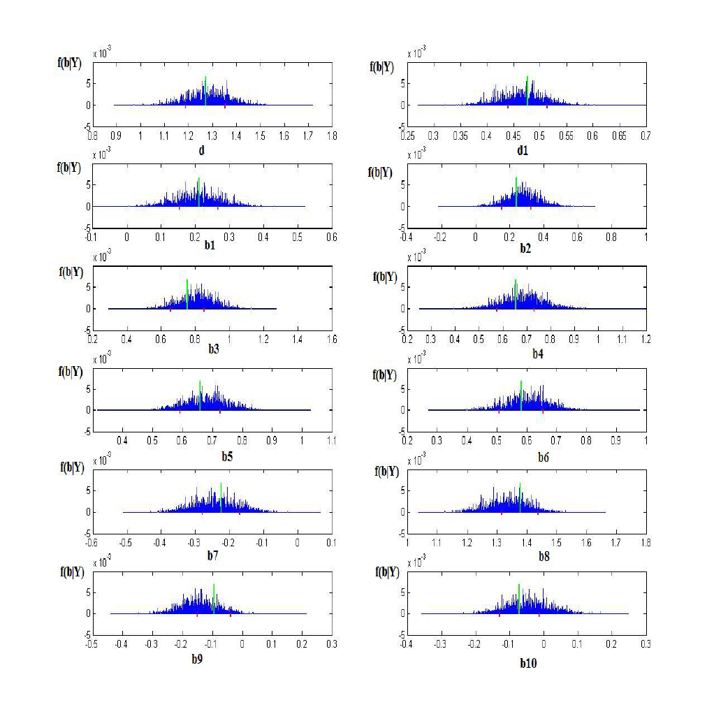
To calculate the standard deviation of the parameters without knowing the distribution of the a
posteriori law, we assume that this standard deviation is equal to the half of the length between
the first and the last quantile (25% and 75%) of the observations of the a posteriori distribution,
i.e. the 25% of the observations above and below the mode. To this end, we generate values from
the f (β|Y ) a posteriori distribution that we sort and plot according to each parameter of β, i.e.
the refusal, the conflict thresholds and the parameters associated with each level of attribute. In
the appendix 1, we present this graphs for one of the individual models which corresponds to a
person who has chosen at least once each of the four alternatives in the questionnaire. Then we
locate the values of f (β|Y ) corresponding to 25% above and below the f (β|Y ) values associated
with the mode (red lines, appendix 1). We report the values of β ass ociated with the f (β|Y )
of the 25% below and above the mode (green line, appendix 1) to compute the length of each
parameter. The standard deviation corresponds to the half of this length.
The results and the comments of our ”zero” option model by a bayesian approach are given in
the next subsection.
Results and comments
We distinguish the results depending on the overall number of alternatives chosen by an indivi-
dual throughout the questionnaire. For example, if an individual has only selected the options
product h, l and the refusal, the dependent variable is then described with three levels rather
than four. In this case, the individual has not been in a conflict situation along the 20 questions.
Others cases with less than the four levels for the dependent variable also occurred during the
survey. We only present the results of one individual belonging to a sub-sample representing each
case of the dependent variable levels. The comments for a specific sub-sample are valid for all
individuals belonging to it. The individual results are comprised of the estimates, the standard
deviations and the importance of each attribute that are calculated according to the following
equation :
importance of the attribute i =
(maximum − minimum)
of the estimates in the attribute i
P
i
(maximum − minimum)
of the estimates in the attribute i
In the model where people only choose the product h and l without being in a conflict and a
refusal situation, the results of the individual 22 is presented in the appendix 2, table A1.
In this table, we notice that the signs of attribute levels fit expectations. Indeed, the results
demonstrate a preference for the hire length of 48 hours, a quantity of 1000 programmes and
the free access to videos with adverts. Additionally, a website with a maximum of novelties and
a composition of 75% of movies and 25% of series prevails in the individual choices. As for the
trailer, it is not essential in the selection of a VoD website. The attributes that affe ct mainly
the choice of Video on Demand website are the composition according to movies and series,
according to the nove lty of the programmes and the tariff. Indeed, according to the percentage
of importance, thes e attributes are determinant in the Video on Demand website selection. On
the other hand, the quantity of the programmes, the hire length or the availability of the trailers
do not have any importance in the website choice.
The standard deviations are reasonable relative to the estimates, as they are inferior to the
estimated values of the unknown parameters. Finally, we can say that as a whole the es timation
results with the bayesian approach of this individual are satisfactory.
14
The results of the other individuals of this type of model are similar. Therefore, all the com-
ments above can be applied to them. It will be identical when we will present and comment the
other situations according to the dependent variable levels . The same reasoning applies to the
other types of model where the similarities of results across individuals enable us to present and
comment tables for only one individual per model type.
Since the mo del with the explained variable corresponding to the choice of product h and l is
dichotomous, we can also apply the penalized likelihood maximisation. As some softwares like
S-Plus contain the implementation of this estimation procedure, we decide to test it to compare
the results with the bayesian approach since the literature generally re comm ends it in the case
of dichotomous logit model. Thus, we want to know if the properties of the penalized likelihood
estimation suit to our ”zero” option probit specification.
The penalized likelihood estimates of the individual 22 with S-Plus are in the appendix 2, table
A2.
The results derived from the penalized likelihood maximisation are not c onsistent in terms of
signs. For example, the individual 22 shows a negative utility for the level 1000 of the catalogue
attribute, while the level 600 is positive. Yet, it is more likely that the individual 22 prefer to
have 1000 programmes in a VoD website than 600. Additionally, the individual seems to prefer
the paying VoD website to the free one with advert. This observation is also questionable. Also
the video hire length does also not reflect the reality, since its sign shows a preference for the
level 24h rather than 48h.
Moreover, the standard deviations are higher that the estimates. This fact reveals a bad ade-
quacy of the penalized likelihood approach when applied to our ”zero” option sp e cification.
Therefore, the bayesian approach is clearly a better choice.
In the model where the four alternatives are at least chosen once, the results of the bayesian
method are given for the individual 2 in the appendix 3, table A3.
We generally notice that the signs of the co effi cients of this sub-sample as well as their magni-
tude reflect the VoD reality. Besides, the standard errors are appropriate in relative to the size
of the estimates. Indeed, in the case of ordered attributes like the programmes quantity, the hire
length and the tariff between a paying and a free website, it seems logical that an individual
prefer the greatest number of programmes or hire length as well as a website with free videos
rather than having to pay for it. With these bayesian estimates we observe that the level 24h of
the attribute hire length, respectively the level 600 of the attribute quantity, is systematically
inferior to the level 48h, respectively the level 1000 or negative, while 48h, respectively 1000, is
positive. The same asse rtion is possible for the levels free and paying as well as for the levels
free and subscription of the attribute tariff. Indeed, the value of the level free is systematically
superior to the level paying, respectively to the level subscription. Additionally, the subscription
option does not seem to be preferred to the paying one.
The conflict and the refusal coefficients are significant for all individuals of this sub-sample, since
the ratio between the estimates and the standard deviation is large enough (largely greater than

15
2). Indeed, the ratio of the individual 2 is :
refusal ratio =
1.271
0.083
= 15.299
conflict ratio =
0.476
0.036
= 12.929
The significance of the results for the conflict variable confirms the uncertainty of the behaviour
of the consumer facing similar products. Therefore, the introduction of the conflict leads to ad-
ditional information as to the consumer preferences and thus allows to improve the accuracy of
the estimates.
Another general observation concerning this sub-sample is that the attributes with the highest
and most significant importance are the composition, the level of novelties and the tariff. There-
fore, a website offering movie trailers, a great hire length and a great catalogue will not represent
a dec isive product for the consumer. On the contrary, a quantity of programmes close to what
can be found in a video club, the free movies and series (except for the novelties), or a correct
composition of movies and series affect more the consumer behavior in the Video on Demand
choice.
These various assertions demonstrate that our ”ze ro” option model better reflect the real consu-
mer preference and allow us to conclude that the bayesian approach yield consistent and si-
gnificant results in the case of data separation. Additionally, the conflict alternative in the
questionnaire offers people another aspect of the decision making process that exist in reality,
since this option is significant and chosen by a number of individuals. The addition of the conflict
therefore provides supplementary information to the notion of refusal existing in the literature.
In addition to the two previous model types, the dataset also contains individuals having selected
only three options, respectively two, among the four available. The three alternatives model,
respectively the two alternatives model, are, either the product h, l and the refusal, or the
product h, l and the conflict, respective ly the product h and the refusal. We will not comm ent
the results for these sub-samples, as they converge to what has already been said about the four
alternative model. The case of the product h and the refusal option (individual 62) has been
supposed consistent because the individual gives the correct answer to the test question (choice
21
6
) and that his answers are not random.
Additionally, since the variable of this model is dichotomous, we also try to estimate it with the
penalized likelihood maximisation in S-Plus. Unfortunately, this method does not work, since
the X
0
X matrix is not of full rank.
Finally, we present the results of the aggregate model that we use d as an a priori information
for the bayesian approach. These results come from the application of the maximum likelihood
estimation adapted to include each of the models that correspond to the number of alternatives
selected in the questionnaire, into a grouped model to get an overall result. In others words,
we combine the different models into a unique one to obtain the estimation of the unknown
parameters β =
d d1 β
1
. . . β
10
. Indeed, in this aggregate estimation, we associate the
corresponding model and the log-likelihood function with each sub-sample and then make a
6
This question has an obvious answer and is used to assess the consistency of the other answers.
16
grouped estimation of all these models. The results of this aggregate ”zero” option model esti-
mation is presented in the table A4 of the appendix 4.
The aggregate model estimation is carried out on a homogenous population, since all students
are from the same University, in the same degree. Hence, they come from the same social en-
vironment and are approximately in the same age bracket. With heterogenous population, we
should have first created homogenous groups and estimated the model parameters for each group.
The table A5 of the appendix 5 gives the estimates of the model parameters without the refe-
rence level that we have removed to obtain a (X
0
X) full rank matrix. In this table, we show
their t-statistics and their p-values. The estimates of the reference variable are obtained through
the assumption associated with the conjoint analysis, i.e. the com pensation model that is ma-
thematically translated as the sum of the levels of each attribute equal to zero. The reference
variables are in fact the last levels of each attribute :
– catalogue : 600
– website composition : 100% Series
– composition of novelties : only old videos
– tariff : subscription
– hire length : 48 hours
– trailer : none
The aggregate model estimation shows that the concept of ”zero” option, the refusal and the
conflict, are significant. Indeed, their t-statistics are equal 11.638 for the refusal and 8.825 for
the conflict (appendix 5). These values are large enough to conclude with the significance of
these parameters, as confirmed by the 0 p-values. Therefore, the conflict and the refusal offer an
additional explanation to the consumer preference choices of the VoD market and are not irre-
levant in this kind of preference analysis. According to the refusal estimated value, individuals
appreciate products with an utility superior to 1.308, and according to the conflict estimate the
products with an utility difference inferior to 0.471 lead to an uncertainty in the consumer choice.
The attributes of greatest importance are the website composition, the level of novelties and the
tariff. The latter influences significantly the consumer decision making process. The variable of
the highest importance is the website composition. Then, comes the level of novelties, and finally
the tariff. It is suprising that the individuals does not consider the tariff as the most important
characteristic. It means that a well-designed website can be successful even it is paying. However,
the magnitude of the level ”free with advert” is higher than the others, i.e. the composition and
the level of novelties. Therefore, the value associated with the free website has a strong influence
in the calculation of the product utility that contains this level.
As for the quantity of programmes in the catalogue, the hire length and the availability of the
trailer, they are all not conclusive in the VoD website choice according to their importance value.
Additionally, the negative sign of the trailer level shows that this service is more unfavorable
than the opposite. It must be noticed however that the importance value of this variable is not
significant.
The sign and the magnitude of the estimated c oefficients are consistent with the expected reality.
Indeed, for ordered attributes like the quantity of programmes and the hire length, the estimates
are negative for the lower values and positive for the higher ones. Therefore, the lower value of
the hire length (24h), respectively the quantity of programmes (600), is smaller than the highest
one, i.e. 48h for the hire length, res pectively 1000 for the quantity of programmes. The same
17
observation is made between the free and the paying or subscription levels. Indeed, it makes
sens that the parameters associated with the paying or the subscription tariff are lower than
the free video. The estimation results of the coefficients of that attribute tariff reflect this reality.
The estimates for the website composition variable demonstrate preferences in decreasing order
for the level ”75% Movies and 25% Series”, the level ”50% Movies and 50% Series”, and finally
the level ”100% Movies”. Creating a website with only series does not appeal the VoD consumer.
A maximum of novelties is an important criterion in the website choice. However, half of the
novelties available in video clubs is, in terms of satisfaction, close to the maximum of this no-
velties level. On the other hand, a website with only old programmes does not really reflect the
consumer preference in the Video on Demand.
Generally, the estimation results of the ”zero” option aggregate model are c onsistent and satis-
factory from a s tatistical and economic point of view. They reflect well the reality of the Video
on Demand preference. They demonstrate the significance and the importance of the uncertainty
in the choice of similar products (conflict) as well as the indifference of some other VoD web-
sites (refusal). These results allow finally to create VoD websites that better suit the individual
preferences.
In the last subsection, we present the calculation of the market shares for some actual websites
and for an ideal one created based on the estimation results.
Purchase probabilities and market shares
The aggregate e stimation results of our ”zero” option model allow us to determine the attribute
levels that influence the selection of the VoD website. From this information, we create the ideal
website that would satisfy the most. They are made up of the following characteristics :
– Catalogue : 1000 programmes
– Composition : 75% Movies 25% Series
– Novelty : maximum
– Tariff : free advert
– Hire length : 48h
– Availability : none
The aim of the Ideal website creation is in fact to calculate the market shares related to existant
VoD websites. The most popular in France with a composition of movies and series only are
Canalplay and TF1Vision. We select the levels that describe the Canalplay and TF1Vision
websites in order to make them as close as possible to their characteristics from July to November
2006. Some levels are a bit different and inexistant in our level selection, so we opted for the
closer one. For example, TF1Vision in summer 2006 proposed one of their own series free. But,
since most of the programmes are paying, we decide to select the level paying of the attribute
tariff for this website. All the information about the following characteristics are collected from
computer magazines and through direct visit of these websites from July 2006 to November
2006. Thus, Canalplay and TF1Vision are composed of the following levels attributes :
Canalplay
– Catalogue : 1000 programmes
– Composition : 100% Movies

18
– Novelty : half
– Tariff : paying
– Hire length : 24h
– Availability : none
TF1Vision
– Catalogue : 600 programmes
– Composition : 75% Movies 25% Series
– Novelty : half
– Tariff : paying
– Hire length : 24h
– Availability : trailer
According to these website characteristics we can now calculate the individual purchase pro-
babilities in the first place, and the market shares in the second place. The market shares are
deduced either from the individual model or from the aggregate model.
From the individual estimations, we associated with each attribute level for each website their
corresponding estimates. The appendix 8 shows an example for a given individual. The same
procedure is applied to each individual. Then, we calculate the utility u
i
associated with each
website i for each individual by summing the corresponding estimates. The utilities values are
useful to determine the individual purchase probabilities. To this end, two approaches are used,
i.e. the Bradley-Terry-Luce and the logit method. The following equations define them :
Bradley-Terry-Luce :
u
i
P
i
u
i
(23)
logit :
exp(u
i
)
P
i
exp(u
i
)
(24)
Thus, we calculate for each individual the purchase probability according to the Bradley-Terry-
Luce and logit equations. From these values (74 individuals), we observe that they are generally
largely higher for the Ideal website than for the others. Moreover, it seems that both the Canal-
play and TF1Vision websites share out evenly the VoD market since their individual purchase
probabilities are very similar in a market comprised of these three websites
7
.
With these purchase probabilities per individual, we calculate the market shares of each website
by averaging the probabilities :
Market shares =
P
purchase probabilities
individual number (74)
(25)
The market shares derived from the Bradley-Terry-Luce and logit methods are as follows :
Market shares in %
Canalplay TF1Vision Ideal
Bradley-Terry-Luce 16.479 16.127 67.392
logit 7.686 7.568 84.744
7
For example, the Bradley-Terry-Luce probabilities purchases for the individual 2 are : Canalplay
16.77%, TF1Vision 15.65% and Ideal 67.56%. The logit results are : Canalplay 7.85%, TF1Vision 7.45%
and Ideal 84.69%. We will not give the values of the others individuals as they are very similar.

19
We reach the same conclusions as with the individual purchase probabilities, i.e. the Ideal sce-
nario offers much higher market shares than Canalplay or TF1Vision whose respective market
shares are very similar.
However, the market shares calculated with the individual purchase probabilities does not take
into account the refusal and the conflict. We consider these situations only with the aggregate
market share calculation. The reason is that we can only obtain the aggregate utilities of the
websites with the aggregate model and compare them to the refusal and conflict thresholds. In
the individual case we can not have the correct aggregate utilities considering the incomparable
measurement scales.
As for the market shares computed from the aggregate model, we obtain them by calculating
the scenario utilities from the aggregate maximum likelihood estimates :
Utilities Refusal
Canalplay TF1Vision Ideal δ
0.749 1.021 3.053 1.308
These estimated utilities can be used to determine the products that are not appreciated by the
consumers. On the other hand, the utility differences can be used to detect a conflict situation :
Difference Conflict
Canalplay-Tf1Vision Canalplay-Ideal TF1Vision-Ideal δ
0
0.271 2.303 2.031 0.471
According to the tabulated values, we notice that the Canalplay and TF1Vision websites are in
the refusal area since their utilities are inferior to δ. Therefore, in a market where the Canalplay,
TF1Vision and Ideal websites coexist, the Canalplay and TF1Vision products are not selected by
the consumers and only the Ideal VoD website represents an interesting option leading to 100%
market shares. Additionally, according to the values of the differences, it seems that Canalplay
and TF1Vision products create difficulties to decide between them because of their similarities.
Indeed, the difference between the Canalplay and TF1Vision websites is inferior to the δ
0
value
that represents the conflict.
A 100% market share does not provide any information about the Canalplay and TF1Vision
influences on the Video on Demand market. So we decide to calculate the purchase influences
in a market with only Canalplay and TF1Vision. Because we only compare two sce narios in
our market, with the equations (1), (2), (3) and (4) we can directly calculate the Canalplay,
TF1Vision, refusal and conflict probabilities
8
.
By inserting in the above mentioned equations the estimates resulting from the aggregate maxi-
mum likelihood estimation, we obtain the following results :
Probabilities
Canalplay TF1Vision Refusal Conflict
0.186 0.291 0.436 0.085
We observe that the refusal probability is high but way below 100%, i.e. it does not suppose
that the Canalplay and TF1Vision products are not appreciated by the consumers. Indeed,
they have market shares superior to 0% when they coexist in a same market. In fact, on 100
8
where σ is set to 1 to take into account the parameters identification.

20
individuals, 19 select C analplay, 29 TF1Vision, 44 do not like the products and 8 do not reach
any decision about their website preferences. To take into account refusal and conflict situations,
we still must transform these probabilities to obtain the real market shares. Indeed, the 44%
in the refusal area do e s not correspond to potential customers and therefore must be excluded
from the market share calculations. The 8% are shared out evenly among the Canalplay and the
TF1Vision products because of the consumer uncertainty. Because the refusal probability has
been removed, we must readjust the Canalplay and TF1Vision probabilities to obtain a sum of
probabilities equal to 100% in the following way :
Probability with conflict
Canalplay TF1Vision
0.186+0.0428 0.291+0.042
=0.229 =0.334
Sum of the probabilities with conflict
0.563
Market shares
Canalplay TF1Vision
0.229
0.563
=
0.334
0.563
=
0.407 0.592
This method that takes account of the refusal and the conflict shows that in a market where
there are only individuals interested in the Canalplay and TF1Vision websites, the market shares
reach 40.71% for Canalplay and 59.29% for TF1Vision. The market shares of TF1Vision website
are here higher than Canalplay. This result demonstrates that the refusal and the conflict are
a source of additional information in the behavioral understanding of the decision making pro-
cess. Indeed, our ”zero” option specification allows us, for the market shares calculation, to take
only into account the potential consumers and to insert people who hesitate in their choices.
Therefore, our market shares truly represent the consumers that are potentially ready to buy
the type of products proposed.
CONCLUSION
In this paper, we present a new specification of the ”zero” option defined in the literature as an
inappreciation of products (refusal) and that is not tackled in details. Additionally, we add to
this refusal a new element, called conflict. The latter takes into account the c ase of uncertainty
during the decision making process due to similarities in the products. Our specification relates
to a model of pair comparisons to which we add the two concepts of the ”zero” option, i.e. the
refusal and the conflict. Indeed, the addition of the refusal, respectively the conflict, is done
by adding to the pair comparison the option ”I do not like any product”, respectively ”I like
both products”. Our model is in fact a mix of the ordered response and the utility comparison
models. The utility comparison model is implemented by defining the products with an utility
and by comparing them. As for the ordered response model, it is used to describe the refusal and
the conflict by thresholds that are compared to the products utilities. The reason of this models
mix is that the utility maximisation do es not consider the conflict in its estimation process.
Additionally, an utility associated with the no choice is not really interpretable as it would be
for products.
Because our ”zero” option model is specified by a probit choice s tructure, we estimate the unk-
nown parameters with the maximum likelihood m ethod. This procedure can run into convergence
troubles with small data size leading to the divergence of the model. We can resolve it by using
21
other alternatives. The two that we have presented in our paper are the bayesian approach and
the penalized likelihood estimation.
To illustrate our ”zero” option model, we undertake an application to the Video on Demand
(VoD) websites. We analyse our specification in the individual and aggregate case. The aggregate
model is estimated with the maximum likelihood. The same approach is not possible with the
individual case because of the small data size leading to infinite estimates of the model. To solve
it we use the bayesian approach. The results are satisfactory from a statistical and economic
point of view. It shows a strong influence of the website composition in terms of movies and se-
ries, the novelties level as well as the hiring cost. For the tariff, the free video with advert prevail
over the paying or subscription option. The consumers also prefer a VoD website composition
with 75% Movies and 25% Series. They do not like websites with only old programmes. They
prefer a mix with the new and old videos with a slight preference for the composition with a
maximum of novelties. The services like the trailer availability, the programmes quantity and
the hire length are not significant.
As for the refusal and the conflict, our application shows that the parameters associated with
the no choice are significant. Therefore, the conflict and the refusal addition is really important
because of the supplemental information it conveys about the individual behavior in the decision
making process.
According to our empirical example we demonstrate that the bayesian approach in the di-
chotomous case offers better results from a statistical and economic point of view than the
widespread penalized likelihood estimation. The latter that is recommended in the literature
for the dichotomous logit model with data separation does not have the same effect with our
probit specification. Therefore, our decision to use a bayesian approach has been conclusive and
demonstrates that the penalized likelihood is not adapted to every model.
We also calculate the market shares of two existing French VoD websites, Canalplay and TF1-
Vision, that are compared to one that is created in such a way that it reflects the consumer
preferences. In a market with those three websites, we observe that the existing ones are in the
refusal area. This means that they are not appreciated by the consumers. Additionally, had they
been selected, they are too similar and lead to uncertainty of choice about these products. The
introduction of the conflict has therefore an advantage as illustrated in this example in that it en-
ables competitors whose offer is similar, to come up with this little something that will make the
difference. For example, if one of the websites offers a gift or an additional free service, it could
orientate the consumer towards its VoD website. We also test the market with only the existing
French websites, Canalplay and TF1Vision. The market shares show a preference for TF1Vision.
In conclusion, we have specified a ”zero” option model that includes the refusal and the conflict
and have demonstrated the importance to insert the conflict in the decision making process
model. An interesting analysis that has not been conducted in this work is to compare our
specification to others like the pair comparison model without the refusal and the conflict, or
the pair comparison model with the refusal only and vice versa. From an econometric and coding
point of view, other perspectives could be implemented, like a logit specification of our ”zero”
option model that could be estimated with the bayesian and the penalized likelihood approaches
to define which one gives better results. With this end in view, the maximum penalized likelihood
should be available in a commercial software. The programming of this procedure could be in
fact very interesting for the users.
The extension of our ”zero” option model to a triple comparison of the products with the inser-
22
tion of the refusal and the conflict could also be of interest. However, the graphical construction
would be more complex as well as the development of the probabilities associated with the five
alternatives proposed in the questionnaire.
23
APPENDIX
Appendix 1
Figure A1
GRAPHS OF THE A POSTERIORI GENERATE DISTRIBUTION (f (β|Y )) FOR EACH
MODEL PARAMETER
where d correspond to the refusal threshold denoted in the text δ, d1 to the conflict threshold
denoted in the text δ
0
and b1 − b10 to the parameter β
1
− β
10
the parameters associated with
each level of each attribute.
24
Appendix 2
Table A1
RESULTS FROM THE BAYESIAN APPROACH OF THE MODEL WITH ONLY TWO OF
THE FOUR ALTERNATIVES SELECTED (THE PRODUCT h AND l)
Individual 22
Variable Utility Standard Error Importance
(% Utility Range)
Catalogue : 1000 0.173 0.069 4.32%
Catalogue : 600 -0.173 0.069
Composition : 100% Movies 0.315 0.095 33.82%
Composition : 75% Movies 25% Series 0.858 0.102
Composition : 50% Movies 50% Series 0.676 0.076
Composition : 100% Series -1.850 0.274
Novelty : max 0.702 0.061 25.46%
Novelty : half 0.633 0.059
Old : max -1.336 0.121
Tariff : paying -0.224 0.054 31.54%
Tariff : free advert 1.375 0.059
Tariff : subscription -1.150 0.113
Hire length : 24h -0.120 0.052 2.99%
Hire length : 48h 0.120 0.052
Availability : trailer -0.073 0.059 1.84%
Availability : None 0.073 0.059
25
Table A2
RESULTS FROM THE PENALIZED LIKELIHOOD APPROACH OF THE MODEL WITH
ONLY TWO OF THE FOUR ALTERNATIVES SELECTED (THE PRODUCT h AND l )
Individual 22
Variable Utility Standard Error Importance
(% Utility Range)
Catalogue : 1000 -0.792 1.127 9.52%
Catalogue : 600 0.792 1.127
Composition : 100% Movies -0.626 1.960 36.76%
Composition : 75% Movies 25% Series -1.976 1.890
Composition : 50% Movies 50% Series -1.528 1.754
Composition : 100% Series 4.131 5.605
Novelty : max -2.172 1.411 37.07%
Novelty : half -1.816 1.141
Old : max 3.988 2.553
Tariff : paying 0.334 1.273 5.42%
Tariff : free advert -0.579 1.045
Tariff : subscription 0.245 2.319
Hire length : 24h 0.698 1.119 8.31%
Hire length : 48h -0.698 1.119
Availability : trailer 0.242 1.092 2.89%
Availability : none -0.242 1.092
Likelihood ratio test=9.925 on 10 df, p=0.447, n=20
26
Appendix 3
Table A3
RESULTS FROM THE BAYESIAN APPROACH OF THE MODEL WITH THE FOUR
ALTERNATIVES SELECTED (THE PRODUCT h, l, THE REFUSAL AND THE
CONFLICT)
Individual 2
Variable Utility Standard Error Importance
(% Utility Range)
Refusal : δ 1.271 0.083
Conflict : δ
0
0.476 0.036
Catalogue : 1000 0.210 0.056 5.55%
Catalogue : 600 -0.210 0.056
Composition : 100% Movies 0.240 0.084 31.63%
Composition : 75% Movies 25% Series 0.751 0.097
Composition : 50% Movies 50% Series 0.654 0.078
Composition : 100% Series -1.645 0.260
Novelty : max 0.658 0.067 25.05%
Novelty : half 0.581 0.073
Old : max -1.240 0.140
Tariff : paying -0.224 0.054 33.39%
Tariff : free advert 1.377 0.060
Tariff : subscription -1.153 0.114
Hire length : 24h -0.094 0.056 2.48%
Hire length : 48h 0.094 0.056
Availability : trailer -0.071 0.058 1.88%
Availability : None 0.071 0.058
27
Appendix 4
Table A4
RESULTS FROM THE MAXIMUM LIKELIHOOD ESTIMATION OF THE AGGREGATE
MODEL
Aggregate model
Variable Utility Standard Error Importance
(% Utility Range)
Refusal : δ 1.308 0.112
Conflict : δ
0
0.471 0.053
Catalogue : 1000 0.212 0.085 3.14%
Catalogue : 600 -0.212 0.085
Composition : 100% Movies 0.262 0.121 35.51%
Composition : 75% Movies 25% Series 0.800 0.128
Composition : 50% Movies 50% Series 0.676 0.112
Composition : 100% Series -1.597 0.362
Novelty : max 0.690 0.090 29.71%
Novelty : half 0.625 0.088
Old : max -1.315 0.178
Tariff : paying -0.235 0.079 23.49%
Tariff : free advert 1.350 0.081
Tariff : subscription -1.115 0.160
Hire length : 24h -0.114 0.078 3.39%
Hire length : 48h 0.114 0.078
Availability : trailer -0.053 0.082 1.58%
Availability : None 0.053 0.082
28
Appendix 5
Table A5
RESULTS FROM THE MAXIMUM LIKELIHOOD ESTIMATION OF THE AGGREGATE
MODEL WITHOUT THE ATTRIBUTE REFERENCE LEVELS
CONVERGENCE ACHIEVED AFTER 19 ITERATIONS
618 FUNCTION EVALUATIONS
Standard
Parameter Estimate Error t-statistic P-value
D 1.308 0.112 11.638 [0.000]
D1 0.471 0.053 8.825 [0.000]
B1 0.212 0.085 2.493 [0.013]
B2 0.262 0.121 2.163 [0.030]
B3 0.800 0.128 6.239 [0.000]
B4 0.676 0.112 6.009 [0.000]
B5 0.690 0.090 7.659 [0.000]
B6 0.625 0.088 7.080 [0.000]
B7 -0.235 0.079 -2.965 [0.003]
B8 1.350 0.081 16.615 [0.000]
B9 -0.114 0.078 -1.450 [0.147]
B10 -0.053 0.082 -0.648 [0.516]
where
D Refusal
D1 Conflict
B1 Catalogue : 1000
B2 Composition : 100% Movies
B3 Composition : 75% Movies 25% Series
B4 Composition : 50% Movies 50% Series
B5 Novelty : max
B6 Novelty : half
B7 Tariff : paying
B8 Tariff : free advert
B9 Hire length : 24h
B10 Availability : trailer

29
Appendix 6
Table A6
ESTIMATES AND UTILITIES OF THE CANALPLAY WEBSITE
Individual 2
Canalplay Attributes Levels Estimates
Catalogue 1000 0.210
Composition 100% Movies 0.240
Novelty half 0.581
Tariff paying -0.224
Hire length 24h -0.094
Availability none 0.071
Utility u
i
i=Canalplay Sum of the estimates 0.785
=Canalplay website utility
for the individual 2
Individual purchase
u
i
i
u
i
(Bradley-Terry-Luce) 16.773%
probabilities in %
exp(u
i
)
i
exp(u
i
)
(logit) 7.850%
Table A7
ESTIMATES AND UTILITIES OF THE TF1VISION WEBSITE
Individual 2
TF1Vision Attributes Levels Estimates
Catalogue 600 -0.210
Composition 75% Movies 25% Series 0.751
Novelty half 0.581
Tariff paying -0.224
Hire length 24h -0.094
Availability trailer -0.071
Utility u
i
i=TF1Vision Sum of the estimates 0.733
=TF1Vision website utility
for the individual 2
Individual purchase
u
i
i
u
i
(Bradley-Terry-Luce) 15.657%
probabilities in %
exp(u
i
)
i
exp(u
i
)
(logit) 7.451%
Table A8
ESTIMATES AND UTILITIES OF THE IDEAL WEBSITE
Individual 2
Ideal Attributes Levels Estimates
Catalogue 600 0.210
Composition 75% Movies 25% Series 0.751
Novelty half 0.658
Tariff paying 1.377
Hire length 24h 0.094
Availability trailer 0.071
Utility u
i
i=Ideal Sum of the estimates 3.163
=Ideal website utility
for the individual 2
Individual purchase
u
i
i
u
i
(Bradley-Terry-Luce) 67.568%
probabilities in %
exp(u
i
)
i
exp(u
i
)
(logit) 84.697%
30
REFERENCES
(2000), ”Preference Structure Measurement : Conjoint Analysis and Related Techniques : A
Guide for Designing and Interpreting Conjoint Studies”, Second Edition, Intelligest
Altman M., Gill J., and McDonald M. P. (2004), ”Numerical issues in statistical computing
for the social scientist”, Chapter 10 : Convergence Problems in Logistic Regression, Allison P.,
Wiley
Bagozzi R. P. (1994), ”Advanced Methods of Marketing Research”, Blackwell Business
Baron J. and Ritov I. (1994), ”Reference Points and Omission Bias”, Organizational Behavior
and Human Decision Processes, 59 (September), 475-498
Beattie J. and Barlas S. (1992), ”Predicting Perceived Differences in Tradeoff Difficulty”, working
paper, University of Sussex
Ben-Akiva M. and Lerman S. R. (1985), Discrete Choice Analysis : Theory and application to
travel demand, Mit Press, Cambridge, MA
Benammou S., Saporta G., and Swissi B. (2007), ”Une proc´edure de r´eduction du nombre de
paires en analyse conjointe”, Journal de la Soci´et´e Fran¸caise de Statistique, tome 148, n
◦
4
Bull S. B., Mak C., and Greenwood C. M. T. (2002), ”A modified score function estimator for
multinomial logistic regression in small samples”, Computational Statistics and Data Analysis,
39, 57-74
Congdon P. (2001), ”Bayesian Statistical Modelling, Chichester, UK : John Wiley
Dagnelie P. (2003), Principe d’exp´erimentation : Planification des exp´eriences et analyse de leurs
r´esultats, Les presses agronomiques de Gembloux
Dhar R. (1997), ”Consumer Preference for a No-Choice Option”, Journal of Consumer Research,
Vol. 24, Septembre
Dussaix A.-M., Saporta G., Carle P., Darmon R.-Y., Grimmer J.-F., and Morineau A. (1998),
”L’Analyse Conjointe, la Statistique et le Produit Id´eal : M´ethodes et Applications, Cisia·Ceresta
Elrod T., Louviere J. J., and Krishnakumar S. D. (1992), ”An Empirical Comparison of Ratings-
Based and Choice-Based Conjoint Models”, Journal of Marketing Research, Vol. XXIX, Aoˆut
Evrard Y., Pras B. , and Roux E. (2003), ”MARKET : Etudes et Recherches en Marketing”, 3
e
Edition, Dunod
Faivre J.-Ph. and Pioche A. (1976), ”L’Analyse des D´ecisions d’Achat par le Mod`ele Trade-off :
Probl`emes Th´eoriques et M´ethodologiques”, Revue Fran¸caise du Marketing, Cahiers 64-65
Festinger L. (1964), ”Conflict, Decision an Dissonance”, Stanford University Press
Firth D. (1993), ”Bias reduction of maximum likelihood estimates”, Biometrika, 80, 1, pp. 27-38
Furlan R. and Corradetti R. (2004), ”An Empirical Comparison of Conjoint Analysis Models
on a Same Sample”, Giornata di Studio ”La Conjoint Analysis” 27 septembre 2004, Universita
degli Studi Salerno

31
Galindo-Garre F., J. K. Vermunt, and W. P. Bergsma (2004), ”Bayesian Posterior Estimation
of Logit Parameters with Small Samples”, Sociological Methods and Research, Vol. 33, No 1,
88-117
Greene W. H. (1993), ”Econometrics analysis”, Fifth Edition, Prentice Hall
Gustafsson A., Herrmann A. , and Huber F. (2003), ”Conjoint Measurement : Methods and
Applications”, Third Edition, Springer
Haaijer M. E. (1999), ”Modeling Conjoint Choice Experiments with the Probit Model”, Labyrint
Publications
Harbi S. (2004), Sur Diff´erentes Approches Multidimensionnelles de Liaisons entre Deux En-
sembles et leurs Applications `a l’Analyse Conjointe : R´egression PLS / Approche du PCAR,
Th`ese, Universit´e de Tunis El Manar, Facult´e de Sciences Economiques et de Gestion de Tunis,
Sous la Direction des Professeurs Gilbert Saporta e t Samir Ben Ammou
Heinze G. (2006), ”A comparative investigation of methods for logistic regression with separated
or nearly separated data”, Statistics in Medecine, 25, 4216-4226
Heinze G. and Ploner M. (2004), ”Technical Report 2/2004 : A SAS macro, S-PLUS library
and R package to perform logistic regression without convergence problems”, Section of Clinical
Biometrics, Department of Medical Computer Sciences, Medical University of Vienna, Vienna,
http ://www.meduniwien.ac.at/msi/biometrie/programme/fl/tr2 2004.pdf
Heinze G. and Ploner M. (2003), ”Fixing the nonconvergence bug in logistic regression with
SPLUS and SAS”, Computer Methods and Programs in Biomedicine, 71, 181-187
Heinze G. and Schemper M. (2002), ”A solution to the problem of separation in logistic regres-
sion”, Statistics in Medicine, 21, 2409-2419
Janis I. L. and Mann L. (1977), ”Decision Making”, New York : Free Press
Johnson R. M. (1997), ”Individual Utilities from Choice Data : a New Me thod”, Sawtooth
Software Conference Proceedings
Johnson R. M. (1997), ”ICE : Individual Choice Estimation”, Technical Paper Series, Sawtooth
Software, Inc.
Karni E. and Schwarz A. (1977), ”Search Theory : The Case of Search with Uncertain Recall”,
Journal of Economic Theory, 16 (October), 38-52
Cite this article as : Roselinde Kessels, Peter Goos, and Martina Vandebroek, ”Optimal designs
for conjoint experiments”, Computational Statistics and Data Analysis (2007), doi : 10.1016/j.csda.2007.10.016
Kuhl J. (1986), ”Human Motivation : From Decision Making to Action Control”, in New Di-
rections in Research on Decis ion Making, ed. B. Brehmer, H. Jungermann, P. Lourens, and G.
Sevon, Amsterdam : North-Holland
Kuhfeld W. F. (2005), ”Marketing Research Methods in SAS : Experimental Design, Choice,
Conjoint, and Graphical Techniques”, SAS 9.1 Edition, SAS Institute Inc., Cary, NC, USA,
http ://support.sas.com/techsup/technote/ts722.pdf
32
Liquet J.-C. (2001), ”Cas d’Analyse Conjointe”, Editions TEC&DOC
Lollivier S. (2006), ”Econom´etrie avanc´ee des variables qualitatives”, Economica
Louviere J. J. (1988), ”Analyzing Individual Decision Making : Metric Conjoint Analysis”, Sage
University Series on Quantitative Applications in the Social Sciences, Series No. 67, Newbury
Park, Ca : Sage Publications , Inc.
Louviere J. J., Hensher D. A., and Swait J. D. (2000), ”Stated Choice Methods : Analysis and
Application”, Cambridge University Press
Maddala G. S. (1983), Limited Dependent and Qualitative Variables in Econometrics, Cambridge
University Press
Mehta C. R., Patel N. R. (1995), ”Exact Logistic regression : theory and examples”, Statistics
in Medicine, vol. 14, 2143-2160,
Montgomery D. C. (1976), Design and Analysis of Experiments, Second Edition, Wiley
Montgomery H. (1989), ”From Cognition to Action : The Search for Dominance in Decision
Making”, in Process and Structure in Human Decision Making, e d. Henry Montgomery and Ola
Svenson, New York : Wiley
Orme B. (2000), ”Hierarchical Bayes : Why All the Attention ?”, Research Paper Series, Saw-
tooth Software, Inc.
Ritov I. and Baron J. (1990), ”Reluctance to Vaccinate : Omission Bias and Ambiguity”, Journal
of Behavioral Decision Making, 3 (December), 263-277
Saporta G. (2006), ”Probabilit´es, analyse des donn´ees et statistique”, 2`eme ´edition, Technip
Scholnick E. K. and Wing C. S. (1988), ”Knowing When You Don’t Know : Developmental and
Situational Considerations”, Developmental Psychology, 24 (March), 190-196
Sjoberg L. (1980), ”Volitional Problems in Carrying through through a Difficult Decision”, Acta
Psychologica, 12 (August), 123-132
Spranca M., Minsk E., and J. Baron (1991), ”Omission and Commission in Judgment and
Choice”, Journal of Experimental Social Psychology, 27 (January), 76-105
Thomas A.(2000), ”Econom´etrie des variables qualitatives”, Dunod
Tversky A. and Shafir E. (1992), ”Choice under Conflict : The Dynamics of Deferred Dec ision”,
Psychological Science, Vol. 3, No 6 (November), 358-361
Zorn C. (2005), ”A solution to separation in binary response models”, Political Analysis, Volume
13, Number 2, 157-170
The computer French magazines : L’Ordinateur Individuel, P2PMag, Micro Actuel, Micro hebdo
Some newspapers : Le Monde, Le Temps
Some websites : LExpansion.com, Wikip´edia, linternaute.com, www.ratiatum.com
