
NOTES AND SOLUTIONS TO THERMAL PHYSICS BY CHARLES KITTLE AND HERBERT KROEMER
ERNEST YEUNG - LOS ANGELES
ABSTRACT. These are notes and solutions to Kittle and Kroemer’s Thermal Physics. The solutions are (almost) complete: I will
continuously add to subsections, before the problems in each chapter, my notes that I write down as I read (and continuously reread).
I am attempting a manifold formulation of the equilibrium states in the style of Schutz’s Geometrical Methods of Mathematical
Physics and will point out how it applies directly to Thermal Physics. Other useful references along this avenue of investigation is
provided at the very bottom in the references.
Any and all feedback, including negative feedback, is welcomed and you can reach me by email or my wordpress.com blog.
You are free to copy, edit, paste, and add onto the pdf and LaTeX files as you like in the spirit of open-source software. You are
responsible adults to use these notes and solutions as governed by the Caltech Honor Code: “No member of the Caltech community
shall take unfair advantage of any other member of the Caltech community” and follow the Honor Code in spirit.
SECOND EDITION. Thermal Physics. Charles Kittel. Herbert Kroemer. W. H. Freeman and Company. New York.
QC311.5.K52 1980 536’.7 ISBN 0-7167-1088-9
1. STATES OF A MODEL SYSTEM
2. ENTROPY AND TEMPERATURE
Thermal Equilibrium. EY : 20150821 Based on considering the physical setup of two systems that can only exchange
energy between each other, that are in thermal contact, this is a derivation of temperature.
U = U
1
+ U
2
is constant total energy of 2 systems 1, 2 in thermal contact
multiplicity g(N, U) of combined system is
g(N, U) =
X
U
1
≤U
g
1
(N
1
, U
1
)g
2
(N
2
, U − U
1
)
The “differential” of g(N, U ) is
dg =
∂g
1
∂U
1
N
1
g
2
dU + g
1
∂g
2
∂U
2
N
2
dU
2
= 0
EY : 20150821 This step can be made mathematically sensible by considering the exterior derivative d of g ∈ C
∞
(Σ), where
Σ is the manifold of states of the system, with local coordinates N, U, where U happens to be a global coordinate. Then,
consider a curve in Σ s.t. it has no component in
∂
∂N
,
∂
∂N
1
, and this curve is a “null curve” so that the vector field X ∈ X(Σ)
generated by this curve is s.t. dg(X) = 0.
With −dU
1
= dU
2
,
1
g
1
∂g
1
∂U
1
N
1
=
1
g
2
∂g
2
∂U
2
N
2
=⇒
∂ ln g
1
∂U
1
N
1
=
∂ ln g
2
∂U
2
N
2
Define
σ(N, U) := ln g(N, U)
Then
=⇒
∂σ
1
∂U
1
N
1
=
∂σ
2
∂U
2
N
2
Date: Fall 2008.
I am crowdfunding on Tilt/Open to support basic sciences research: ernestyalumni.tilt.com. If you find this pdf (and LaTeX file) valuable
and/or helpful, please consider donating to my crowdfunding campaign. There is also a Paypal button there and it’s easy to donate with PayPal, as I had
recently to the Memorial Fund for the creator of Python’s matplotlib. But the most important thing is for anyone, anywhere, and at anytime be able to
learn thermodynamics and use it for research and application and so I want to keep this as openly public as possible, in the spirit of open-source software.
Tilt/Open is an open-source crowdfunding platform that is unique in that it offers open-source tools for building a crowdfunding campaign. Tilt/Open has
been used by Microsoft and Dicks Sporting Goods to crowdfund their respective charity causes.
1

Temperature. T
1
= T
2
- temperatures of 2 systems in thermal equilibrium are equal.
T “must be a function of
∂σ
∂U
N
[?].
=⇒
1
T
= k
B
∂σ
∂U
N
Experimentally, k
B
= 1.381 × 10
−23
J/K = 1.381 × 10
−16
ergs/K.
Now
1
τ
=
∂σ
∂U
N
τ = k
B
T
Problems. Solution 1. Entropy and temperature.
(a) Recall that
1
τ
≡
∂σ
∂U
N,V
and σ(N, U) ≡ log g(N, U). Given g(U ) = CU
3N/2
,
σ(N, U) = log CU
3N/2
= log C +
3N
2
log U
∂σ
∂U
=
3N
2
1
U
=
1
τ
=⇒ U =
3N
2
τ
(b)
∂
2
σ
∂U
2
N
< 0 ?
∂
2
σ
∂U
2
N
= −
3N
2
1
U
2
< 0
Solution 2. Paramagnetism.
U(s) = U
1
(s
1
) + U
2
(s
2
) = −2mB(s
1
+ s
2
) = −2mBs or s =
U
−2mB
i.e. potential energy U(s) = −2s · mB.
For |s| N, then
g(N, s) ' g(N, 0) exp
−2s
2
/N
= g(N, 0) exp
−U
2
2(mB)
2
N
σ(N, U) = ln g(N, U) = σ
0
−
U
2
2m
2
B
2
1
N
where σ
0
= ln g(N, 0)
1
τ
=
∂σ
∂U
N
=
−U
m
2
B
2
1
N
What is the thermal equilibrium value of this N -spin system of fractional magnetization? If U denotes hUi, thermal average
energy, we also get the thermal average spin excess.
hUi = h−2mBsi = −2mBhsi
=⇒ τ =
m
2
B
2
N
−U
=
mBN
2hsi
Solution 3. Quantum harmonic oscillator.
(a) Result from Ch. 1: g(N, n) =
(N+n−1)!
n!(N−1)!
.
Let N − 1 → N =⇒ g(N + 1, n) =
(N+n)!
n!N!
.
σ(N + 1, n) ≡ ln g(N + 1, n) = ln
(N + n)!
n!N!
= ln (N + n)! − ln (n!) − ln (N!)
≈ (N + n) ln (N + n) − N −n − n ln n + n − N ln N + N = (N + n) ln (N + n) − n ln n −N ln N
(b) Let U denote total energy n~ω of oscillators.
U = n~ω or n =
U
~ω
σ(N, U) = (N +
U
ω
) ln (N +
U
ω
) −
U
ω
ln
U
ω
− N ln N
At τ,
1
τ
=
∂σ
∂U
N
.
1
τ
=
1
ω
ln (N +
U
ω
) −
1
ω
ln
U
ω
=
1
ω
ln
Nω
U
+ 1
or U =
Nω
exp (ω/τ) − 1
2

Solution 4. The meaning of “never.”
Suppose 10
10
monkeys.
(a) Hamlet represents one specific ordering of 10
15
with 44 possibilities for each character. The probability of hitting
upon Hamlet from a given, random sequence is
1
44
100000
=
1
44
100000
. Given that log
10
44 = 1.64345, then
10
1.64345
= 44 or 10
−1.64345
= 44
−1
so then
1
44
100000
= 10
−164345
(b)
(age of universe) ·
10 keys
second
= 10
18
s
10 keys
second
= 10
19
keys
10
19
keys · 10
10
monkeys = 10
29
keys typed out
1 hamlet
10
5
characters
= 10
24
possible “Hamlets”
From part (a), the probability that a given, random sequence is Hamlet, 10
−164345
(10
29
characters)(10
−164345
) = 10
−164316
Note, I think that the probability should be (10
29
characters)
1 Hamlet
10
5
characters
(10
−164345
) = 10
−164321
Since we are considering the number of “Hamlet”, 10
5
character sequences.
3. BOLTZMANN DISTRIBUTION AND HELMHOLTZ FREE ENERGY
cf. Example: Energy and heat capacity of a two state system, pp. 62 of Kittel and Kroemer [1]. Kittel and Kroemer
introduces the heat capacity very early, specific to this example.
Definition 1. heat capacity C
V
at constant volume is defined as
(1) C
V
:= τ
∂σ
∂τ
V
Recall the thermodynamic identity (which is introduced many equations later):
dU = τ dσ −pdV ∈ Ω
1
(Σ)
where Σ is a manifold of states of all systems.
Consider local coordinates of Σ, (σ, V ). Consider curve
c : R → Σ
c(τ) ∈ Σ
s.t. c generates a vector field ˙c = ˙σ
∂
∂σ
i.e. no component
in the V direction. Notice the prescient choice of parameter τ .
Now for internal energy U ∈ C
∞
(Σ), taking the exterior derivative d results in
dU =
∂U
∂σ
dσ +
∂U
∂V
dV
Then applying dU onto vector field ˙σ
∂
∂σ
,
dU
˙σ
∂
∂σ
=
∂U
∂σ
˙σ = ˙στ + 0
Now,
∂U
∂σ
V
∂σ
∂τ
V
=
∂U
∂τ
V
=
∂σ
∂τ
V
τ
Hence,
(2) C
V
:= τ
∂σ
∂τ
V
=
∂U
∂τ
V
EY: 20150825 Why do we need differential geometry? It’s because I always wondered why you could do this:
C
V
:= τ
∂σ
∂τ
V
?
=
∂U
∂τ
V
with τdσ = dU =⇒ τ∂σ
?
= ∂U
and talk of “differentials.”
Definition: Reversible process. EY : 20150824 Mathematically, 1-forms are exact.
3

Pressure. Consider coordinates (σ, V ) ∈ Σ of manifold of thermodynamic states Σ.
Imagine a reversible compression of a cube system (so imagine dV < 0; cube’s volume get smaller).
σ constant, i.e. dσ = 0 (on this curve in Σ) because as particles in cube gets squeezed, less positions particles could sit in,
but they get more kinetic energy, more energetic (more momentum squared).
Now U = U(σ, V ) ∈ C
∞
(Σ).
=⇒ dU =
∂U
∂σ
V
dσ +
∂U
∂V
σ
dV
Again, imagine a curve c : R → Σ, connecting 1 state (σ, V ) ∈ Σ to another state (σ, V + dV ) ∈ Σ s.t. ˙c =
˙
V
∂
∂V
.
=⇒ dU(˙c) =
∂U
∂V
σ
˙
V
Introduce 1-form W ∈ Ω
1
(Σ) of work done on the cube system from some external agent
W = −pdV
so W > 0 when dV < 0.
Then
W ( ˙c) = −p
˙
V = dU ( ˙c) =
∂U
∂V
σ
˙
V
(3) =⇒ p = −
∂U
∂V
σ
Consider another set of coordinates (U, V ) ∈ Σ for manifold Σ. Now entropy σ is a function of U, V , as σ = σ(U, V ) ∈
C
∞
(M), so that
dσ =
∂σ
∂U
V
dU +
∂σ
∂V
U
dV
Consider curve c = (U, V ) ∈ Σ. Then ˙c =
˙
U
∂
∂U
+
˙
V
∂
∂V
. For this curve c, σ is constant, meaning dσ(˙c) = 0 (it’s a “null
curve” of dσ
dσ( ˙c) = 0 =
∂σ
∂U
V
˙
U +
∂σ
∂V
U
˙
V
Now define
Definition 2.
(4)
1
τ
:=
∂σ
∂U
V
So then we have
1
τ
˙
U +
∂σ
∂V
U
˙
V = 0. For the parameter of curve c, choose the parameter to be V , knowing that σ is constant
on this curve, or thermodynamic process. Thus
1
τ
∂U
∂V
σ
= −
∂σ
∂V
U
=⇒
−p
τ
= −
∂σ
∂V
U
or
(5) p = τ
∂σ
∂V
U
Thermodynamic Identity. Let σ = σ(U, V ) ∈ C
∞
(Σ). Then
dσ =
∂σ
∂U
V
dU +
∂σ
∂V
U
dV ∈ Ω
1
(Σ).
Now recall the quantities we’ve recently used:
1
τ
:=
∂σ
∂U
V
(this is a definition) and
p
τ
=
∂σ
∂V
U
(it comes from the physics,
Theorem 1.
(6) τdσ = dU + pdV
Ideal Gas: A First Look.
4

One atom in a box. one atom of mass M in cubical box of volume V = L
3
−~
2
2M
∇
2
ψ = ψ p =
~
i
∇ p
2
ψ = ψ
=⇒ ψ(x) = A sin
n
x
πx
L
sin
n
y
πy
L
sin
n
z
πz
L
n
=
~
2
2M
π
L
2
(n
2
x
+ n
2
y
+ n
2
z
)
Then the partition function Z
1
is
Z
1
=
X
n
exp
−
n
τ
=
X
(n
x
,n
y
,n
z
)
exp
−~
2
2Mτ
π
L
2
(n
2
x
+ n
2
y
+ n
2
z
)
Let
α
2
=
~
2
π
2
2ML
2
τ
or α =
~π
(2Mτ)
1/2
V
2/d
Then
Z
1
=
Z
∞
0
dn
x
Z
∞
0
dn
y
Z
∞
0
dn
z
exp [−α
2
(n
2
x
+ n
2
y
+ n
2
z
)] =
Z
∞
0
dn
x
exp (−α
2
n
2
x
)
3
=
1
α
3
π
1/2
2
3
=
π
1/2
2α
3
In general, Z
1
=
π
1/2
2α
d
Now
Z
1
=
π
1/2
V
1/d
2
~π
(2Mτ )
1/2
!
d
=
V
2~π
Mτ
d/2
= n
Q
V =
n
Q
n
in terms of concentration n = 1/V .
n
Q
:=
Mτ
2π~
2
d/2
is the quantum concentration.
Problems. Solution 1. Free energy of a two state system.
(a)
Z = 1 + e
−/τ
F = −τ ln Z = −τ ln (1 + e
−/τ
)
(b)
U = −τ
2
∂(F/τ)
∂τ
=
e
−/τ
1 + e
−/τ
σ = −
∂F
∂τ
= ln (1 + e
−/τ
) +
τ
e
−/τ
(1 + e
−/τ
)
Solution 2. Magnetic susceptibility
(a) Remember to calculate the multiplicity in the N -spin system (it’s not enough to sum up exp (−
s
/τ) factors).
M = 2sm U
s
= −MB = −2smB N = N
+
+ N
−
2s = N
+
− N
−
= N
+
− (N − N
+
) = 2N
+
− N
Z =
N/2
X
s=−N/2
N
N
+
exp
2smB
τ
=
N/2
X
s=−N/2
N!
N
2
+ s
!
N
2
− s
!
exp
2mBs
τ
=
N
X
s=0
N!
s!(N − s)!
exp
2mB
τ
s −
N
2
=
= e
−
NmB
τ
(1 + e
2mB
τ
)
N
= 2
N
cosh
N
mB
τ
where it was crucial to use (1 + x)
N
=
P
N
j=1
N
j
x
j
. Note, in changing the sum index, since N is large, we can
neglect dropping the s = 0 term.
∂
τ
Z = 2
N
(N)(cosh
N−1
mB
τ
) sinh
mB
τ
−m
τ
2
M = −τ
2
∂
∂τ
ln Z = Nm tanh
mB
τ
χ =
∂M
∂B
=
Nm
2
τ
sech
2
mB
τ
5

(b)
F = −τ ln Z = −τ ln
(2 cosh
mB
τ
)
N
= −Nτ ln (2 cosh
mB
τ
)
For x ≡
M
nm
= tanh
mB
τ
. Now 1 − tanh
2
y = sech
2
y. F = −Nτ ln
2
√
1−x
2
=
−Nτ
2
ln
4
1−x
2
.
(c) For
mB
τ
1, cosh
2
mB
τ
→ 1. χ =
m
2
N
τ
Solution 3. Free energy of a harmonic oscillator
(a)
Z =
∞
X
s=0
exp
−s~ω
0
τ
=
1
1 − e
−~ω
0
/τ
= (1 − e
−~ω
0
/τ
)
−1
F = −τ ln Z = τ ln (1 −e
−~ω
0
/τ
) ' τ ln
~ω
0
τ
for 1
~ω
0
τ
(b)
σ = −
∂F
∂τ
= −{ln (1 − e
−~ω
0
/τ
) +
τ
1 − e
−~ω
0
/τ
(−e
−~ω
0
/τ
)
~ω
0
τ
} =
−~ω
0
/τ
e
~ω
0
/τ
− 1
− ln (1 −e
−
~ω
0
τ
)
Solution 4. Energy fluctuations.
1
τ
= β
∂
∂τ
=
∂β
∂τ
∂
∂β
= −
1
τ
2
∂
∂β
Z =
X
s
e
−
s
β
∂
β
Z =
X
s
−e
−
s
β
∂
2
β
Z =
X
s
2
s
e
−
s
β
U =
P
s
s
e
−
s
/τ
Z
= −∂
β
ln Z
∂U
∂τ
= −β
2
∂
∂β
U = β
2
∂
β
∂
β
Z
Z
= β
2
(∂
2
β
Z)Z − (∂
β
Z)
2
Z
2
!
= β
2
∂
2
β
Z
Z
−
∂
β
Z
Z
2
!
=
=⇒ τ
2
∂U
∂τ
= h
2
i − hi
2
Solution 5. Overhauser effect. System S in energy eigenstate E
n
= n.
P (E) = (1)g
R
(E)
Note ∆U
R
= (α − 1). ∆U
S
= .
dU
S
d
+
dU
R
d
= 1 + (α − 1) = α =
dU
tot
d
in a specific energy eigenstate; g
S
(n) = 1
While g
R
(U
R
) = multiplicity of reservoir R with U
R
energy.
Now
∂σ
R
∂E
s
=
1
τ
and
g
R
(U
R
) = exp (σ
R
(U
R
))
If
dU
R
d
= (α − 1) = ∆U
R
small compared to U
R
.
U
R
(E
S
= (n + 1)) = U
R
(n) +
dU
R
d
= U
R
(n) + (α − 1)
σ
R
(U
R
((n + 1))) ' σ
R
(U
R
(n)) +
1
τ
(α − 1)
P (E
S
= (n + 1))
P (E
S
= n)
=
exp (σ
R
(U
R
(n)) +
1
τ
(α − 1))
exp (σ
R
(U
R
(n)))
= exp
−
τ
(1 − α)
Solution 6. Rotation of diatomic molecules.
(a) (j) = j(j + 1)
0
. g(j) = 2j + 1
Remember that Z is a sum over all states, not over all levels.
Z =
∞
X
j=0
(2j + 1)e
−j(j+1)
0
/τ
=
∞
X
j=0
d
dj
(e
−(j
2
+j)
0
/τ
)
−τ
0
=
−τ
0
∞
X
j=0
d
dj
e
−
0
/τ
j
2
+j
(b) For 1
0
τ
Z
R
(τ) = −
τ
0
Z
∞
0
d
dx
e
−
0
/τ
x
2
+x
dx = −
τ
0
(e
−
0
/τ
)
x
2
+x
− (e
−
0
/τ
)
0
=
τ
0
6

(c) For
τ
0
1
Z
R
(τ) = 1 + 3e
−2
0
/τ
(d)
U = τ
2
∂ ln Z
∂τ
for 1
0
τ
U = τ
2
∂
τ
ln
τ
0
= τ
for
τ
0
1, U = τ
2
1
1 + 3e
−2
0
/τ
(3e
−2
0
/τ
)
2
0
τ
2
=
6
0
e
−2
0
/τ
1 + 3e
−2
0
/τ
C
V
=
∂U
∂τ
V
= 1 when 1
0
τ
C
V
= 6
0
e
−2
0
/τ
2
0
τ
2
(1 + 3e
−2
0
/τ
) − (3e
−2
0
/τ
)
2
0
τ
2
e
−2
0
/τ
(1 + 3e
−2
0
/τ
)
2
!
= 12
2
0
e
−2
0
/τ
τ
2
1
(1 + 3e
−2
0
/τ
)
2
For very small
τ
0
1, C
V
≈ 12
e
−2
0
/τ
(τ/
0
)
2
(e) See sketch.
Solution 7. Zipper problem.
(a) N links.
s
= 0 closed, open.
Z =
N
X
s=0
exp (−s/τ ) =
1 − e
−(N+1)/τ
1 − e
−/τ
(b) 1
τ
.
Z =
P
N
s=0
exp (−sB)
−1
∂
β
ln Z =
−1
P
N
s=0
(−s)e
−sβ
Z
= hsi =
=
1 − e
−/τ
1 − e
−(N+1)/τ
−e
−(N+1)/τ
(−(N + 1))(1 − e
−/τ
) − (−e
−/τ
)(−)(1 − e
−(N+1)//τ
)
(1 − e
−/τ
)
2
=
=
e
−/τ
(e
−Nβ
(N + 1)(1 − e
−β
) − (1 − e
−(N+1)/τ
))
(1 − e
−(N+1)/τ
)(1 − e
−/τ
)
'
e
−/τ
(e
−Nβ
(N + 1)(1 − e
−β
) − 1)
(1 − e
−β
)
This still does not give the desired approximation. Consider the following:
Z =
1 − e
−(N+1)β
1 − e
−β
=
e
β
− e
−Nβ
e
β
− 1
∂
β
Z =
((e
β
+ N βe
−Nβ
)(e
β
− 1) − (e
β
)(e
β
− e
−Nβ
))
(e
β
− 1)
2
=
(e
β
(e
β
+ N e
−Nβ
− e
β
+ e
−Nβ
) − e
β
− N e
−Nβ
)
(e
β
− 1)
2
∂
β
Z
Z
=
(e
β
(N + 1)e
−Nβ
− e
β
− N e
−Nβ
)
(e
β
− 1)(e
β
− e
−Nβ
)
'
(e
β
(N + 1)e
−Nβ
− e
+β
− N e
−Nβ
)
e
2β
=
=
(Ne
−(N−1)β
+ e
−(N−1)β
− e
β
− N e
−Nβ
)
e
2β
=
((N + 1)e
−(N−1)β
− (e
β
+ N e
−Nβ
))
e
2β
=
=
(N+1)e
β
e
Nβ
−
n
e
Nβ
− e
β
e
2β
=
(N+1)e
β
−N
e
Nβ
− e
β
e
2β
=
Ne
β
+e
β
−e
β
e
Nβ
e
Nβ
e
2β
=
N − e
Nβ
e
Nβ
e
β
'
'
(−e
Nβ
)
e
Nβ
e
β
= −e
−β
=⇒ hsi = e
−/τ
Solution 8. Quantum concentration. Now Ψ(x, y, z) = A sin
n
x
πx
L
sin
n
y
πy
L
sin
n
z
πz
L
. p =
1
i
∇,
p
2
2m
= −
1
2m
∇
2
.
Ground orbital: n
x
= n
y
= n
z
= 1.
T =
3
2m
π
L
2
hψ
0
|ψ
0
i =
3
2m
π
L
2
7

where hψ
0
|ψ
0
i = 1, ψ normalized. It was normalized in this way:
Z
∞
0
sin
2
n
x
πx
L
dn
x
=
Z
L
0
1 − cos
2n
x
πx
L
2
dn
x
=
n
x
− sin
2n
x
πx
L
L
2n
x
π
2
L
0
=
L
2
hψ|ψi = A
2
L
2
3
=
A
2
L
3
8
= 1 or A
2
=
8
L
3
Recall that n
Q
=
mτ
2π~
2
3/2
.
Consider the condition that there will be a concentration for which the zero-point quantum kinetic energy is equal to the
temperature τ:
=⇒
3
2m
π
2
L
2
=
3
2m
π
2
n
2/3
= τ or n
2/3
=
2mτ
3π
2
~
2
or n =
2mτ
3π
2
~
2
3/2
=⇒ n = (
4
3π
mτ
2π~
2
)
3/2
=
4
3π
3/2
n
Q
Solution 9. Partition function for two systems.
Z(1 + 2) =
X
E
1+2
g(E
1+2
) exp
−E
1+2
τ
=
X
E
1
+E
2
=E
0
g(E
1
+ E
2
) exp
−E
1
τ
exp
−E
2
τ
=
=
X
E
1
X
E
2
g(E
1
)g(E
2
) exp
−E
1
τ
exp
−E
2
τ
= Z(1)Z(2)
since systems are independent.
Solution 10. Elasticity of polymers.
(a) Consider 2s = N
+
− N
−
; N = N
+
+ N
−
, 2s = N
+
− (N − N
+
) = 2N
+
− N . N
+
=
2s+N
2
.
For 2s, consider −2s = N
+
− (N − N
+
) = 2N
+
− N . N
+
=
−2s+N
2
.
=⇒ g(N, −s) + g(N, s) =
2N!
N
2
+ s
!
N
2
− s
!
(b) |s| N
σ(l) = ln
g
N,
l
2ρ
+ g
N,
−l
2ρ
= ln
2(N!)
N
2
+
l
2ρ
!
N
2
+
−l
2ρ
!
=
= ln (2N !) = {
N
2
+
L
2ρ
ln
N
2
+
l
2ρ
−
N
2
+
l
2ρ
+
N
2
−
l
2ρ
ln
N
2
−
l
2ρ
−
N
2
−
l
2ρ
}
where we used ln(x + ∆x) ' ln x +
1
x
∆x.
σ(l) = ln (2N!) − {
N
2
+
l
2ρ
ln
N
2
+
1
N/2
l
2ρ
−
N
2
+
N
2
−
l
2ρ
ln
N
2
+
1
N/2
−l
2ρ
} =
= ln (2N !) − {
N
2
ln
N
2
−
N
2
+
N
2
ln
N
2
−
N
2
+
l
2ρ
ln
N
2
+
l
2ρ
+
2
N
l
2ρ
2
+
−l
2ρ
−
l
2ρ
ln
N
2
+
l
2
N2ρ
2
}
σ(l) = ln
2N!
N
2
!
N
2
!
!
−
l
2
Nρ
2
(c)
∂σ
∂l
=
−2l
Nρ
2
=⇒ f =
2lτ
Nρ
2
Solution 11. One-dimensional gas.
n
=
~
2
2m
π
L
2
n
2
in one dimension
Z
1
=
∞
X
n=1
exp
−~
2
2m
π
L
2
n
2
/τ
=⇒
Z
∞
0
dne
−α
2
n
2
=
√
π
2α
8

where
α
2
=
~
2
2mτ
π
L
2
α =
~π/L
√
2mτ
1/2
.
Recall that σ =
∂F
∂τ
, F = U − τσ, so that
F = −τ ln Z = −τ N ln
√
π
2α
= τN ln
2α
√
π
= τN ln
2~π/L
√
π
√
2mτ
1/2
=
= τN ln
√
2π~
√
mLτ
1/2
!
=
1
2
τN ln
2π~
2
mL
2
τ
∂F
∂τ
=
1
2
N ln
2π~
2
mL
2
τ
+
τN
2
1
2π~
2
mL
2
τ
!
−2π~
2
mL
2
τ
2
=
=
1
2
N ln
2π~
2
mL
2
τ
+
−τN
2τ
=
N
2
ln
2π~
2
mL
2
τ
− 1
4. THERMAL RADIATION AND PLANCK DISTRIBUTION
Problems. Solution 1. Number of thermal photons.
We consider a cavity of volume V , and of edge length L (so V L
3
). So then ω
n
= nπc/L.
Now
1
exp
(
~ω
n
τ
)
−1
X
hs
n
i =
X
1
exp
~ω
n
τ
− 1
Consider (n
x
, n
y
, n
z
) on positive octant, and 2 independent polarization s of em field.
X
n
1
exp
~nπc
Lτ
− 1
=
(2)
8
Z
∞
0
4πn
2
dn
1
exp
~nπc
Lτ
− 1
= π
Z
∞
0
n
2
dn
exp
~nπc
Lτ
− 1
=
= π
Lτ
~πc
3
Z
∞
0
x
2
dx
e
x
− 1
= N =
V
π
2
τ
~c
3
(2.404)
where I used the substitutions
x =
~πcn
Lτ
Lτx
~πc
= n
(dx)
Lτ
~πc
= dn
Now σ(τ) = (4π
2
V/45)(τ/~c)
3
, so then
σ
N
=
1
2.404
4π
4
45
' 3.602
Now how was
R
∞
0
dx
x
2
dx
e
x
−1
evaluated?
Solution 2. Surface temperature of a Sun. Given the solar constant of the Earth, the total radiant energy flux density at
the Earth from the Sun normal to the incident rays, integrated over all emission wavelengths,
solar constant = 0.136 J s
−1
cm
−2
, (49)
(a)
4π(1.49 × 10
11
m)
2
· 0.136 J s
−1
cm
−2
10
2
cm
1 m
2
= (4π)(1.49)
2
10
22
· 0.136 × 10
4
= 3.8 × 10
26
J · s
−1
Note that I had used 1.49 × 10
11
m as the distance of the Earth from the Sun.
(b) J
ν
= energy flux density or rate of energy emission per unit area.
σ
B
=
π
2
k
4
B
60~
3
c
2
= 5.670 × 10
−8
W m
−2
K
−4
.
Note that W =
1 J
s
. I will use R
◦
= 6.9599 × 10
10
cm as the radius of the Sun.
4 × 10
26
J · s
−1
4π(6.9599 × 10
10
cm)
2
= J
ν
= σ
B
T
4
9

4 × 10
26
J · s
−1
4π(6.9599 × 10
10
cm)
2
1 m
2
10
2
cm
1 m
2
5.670 × 10
−8
J/s
k
4
= T
4
T ' 5830 K
Solution 3. Average temperature of the interior of the Sun.
(a)
U = −
Z
R
0
G
4
3
πρr
3
(4πr
2
ρdr)
r
= −
16
3
π
2
Gρ
2
Z
R
0
r
4
dr =
−16
15
π
2
ρ
2
GR
5
; M =
4
3
πR
3
ρ
U =
−3GM
2
5R
U = −
1
2
Z
R
0
G
4
3
πρr
3
r
(4πr
2
ρdr) =
−8
3
π
2
Gρ
2
Z
R
0
r
4
dr =
−8
15
π
2
ρ
2
GR
5
=
=
−8
15
π
2
GR
5
M
4
3
πR
3
2
=
−3
10
GM
2
R
= 1.14 × 10
41
J
(b) Using the virial theorem of mechanics, note that
−1
2
U =
3
20
GM
2
R
=
3
20
6.67 × 10
−11
kg ·
m
s
2
·
m
2
kg
2
· 2 × 10
33
g
1 kg
10
3
g
7 × 10
10
cm
1 m
10
2
cm
= 5.72 × 10
40
J
Now hsi =
1
exp (~ω/τ )−1
, is the Planck distribution function, giving the thermal average number of photons in a
thermal average energy hi = hsi~ω =
~ω
exp (~ω/τ )−1
for τ ~ω, hi ' τ
So then 5.72 × 10
40
J = Nhi = Nτ.
τ =
5.72 × 10
40
J
1 × 10
57
(1.381 × 10
−23
J/K)
= 4.14 × 10
6
K
Solution 4. Age of the Sun.
(a) Consider 4H →
4
2
He. Then 4(1.0078) − 4.0026 = 0.0286 amu. Then
(0.0286 amu)
1.6726 × 10
−27
kg
1.00727647 u
(3 × 10
8
m/s)
2
= 4.27 × 10
−12
J
Given M
= 2 × 10
3
3 g,
(2 × 10
30
kg)(0.10)
1
4 × (1.0078 amu)
1.00727647 u
1.6726 × 10
−27
kg
(4.27 × 10
−12
J) = 1.28 × 10
44
J
So 1.28 × 10
44
J energy is available.
(b)
1.15 × 10
45
J
4 × 10
26
J · s
−1
1 hr
3600 s
1 day
24 hr
1 yr
365 days
= 1.02 × 10
10
years
Solution 5. Surface temperature of the Earth. J
S
= σ
b
T
4
is the radiant power per unit area.
Total emitted radiation energy of the sun is J
S
4πR
2
.
4πR
2
J
S
4πR
2
ES
=
R
2
R
2
ES
J
S
= radiation energy hitting 1 cm
2
of Earth’s surface in one second
Since the Earth is considered a black-body, the rate of absorption must equal the rate of emission:
R
2
R
2
ES
σ
b
T
4
= σ
b
T
4
e
or T
4
e
= T
4
R
2
=⇒ T
e
= 5800 K
r
7 × 10
10
cm
1.5 × 10
13
cm
= 396.2 K = 123 C
Solution 6. Pressure of thermal radiation.
(a) s
j
= number of photons in that mode. Suppose modes of ω
j
, j = 0, 1, 2, . . . .
j
= s
j
~ω
j
= total energy in jth mode, s
j
photons in jth mode.
U =
X
j
j
=
X
j
s
j
~ω
j
P = −
∂U
∂V
= −
X
j
s
j
~
∂ω
j
∂V
10

(b) ω
j
= jπc/L, V = L
3
. So then ω
j
= jπcV
−1/3
.
=⇒
dω
j
dV
=
−1
3
jπcV
−4/3
=
−1
3
ω
j
V
(c) p =
U
3V
(d) We want the Kinetic pressure at a concentration of (1 mol/cm
3
). Recalling P =
Nk
B
T
V
,
P =
1 mol
cm
3
6.022 × 10
23
1 mol
10
2
cm
1 m
3
1.381 × 10
−23
J
K
(2 × 10
7
K) = 1.663 × 10
14
N
m
2
Now for the thermal radiation pressure,
p =
U
3V
=
1
3
π
2
15~
3
c
3
τ
4
= 4.03 × 10
13
N
m
2
where t = 2 × 10
7
K.
For the pressures to be equal,
1
3
π
2
15~
3
c
3
k
4
B
T
4
=
Nk
B
V
T or T
3
=
45(~c)
3
Nk
B
π
2
k
4
B
V
so that T = 3.2 ×10
7
K
Solution 7. Free energy of a photon gas
(a) Z =
Q
n
1
1−e
−~ω
n
/τ
Consider Z =
P
∞
s=0
e
−s~ω/τ
=
1
1−e
−~ω/τ
for a single mode.
(b) F = −τ ln Z = τ
P
n
ln (1 − e
−~ω
n
/τ
) ω
n
=
nπc
L
.
F = τ
X
n
ln (1 − e
−~ω
n
/τ
) = τ
Z
∞
0
4πn
2
dn
8
(2) ln (1 − e
−~nπc/τL
) = πτ
Z
∞
0
dnn
2
ln (1 − e
−~nπc/τL
) =
= πτ
(n
3
ln (1 − e
−~nπc/τL
))
∞
0
−
Z
∞
0
dn
n
3
e
−~nπc/τL
1 − e
−~nπc/τL
−~πc
τL
= −
~π
2
c
L
Z
∞
0
dn
n
3
e
~nπ/τL
− 1
=
= −
τL
~πc
3
Z
∞
0
x
3
e
x
− 1
= −
(τL)
3
(~
2
c
3
)
π
2
45
where I used x =
~nπc
τL
.
Solution 8. Heat shields. For J
u
= σ
B
(T
4
u
− T
4
l
), the thermal flux without the heat shield, in the middle region. Plane m
absorbs σ
B
T
4
u
+ σ
B
T
4
l
and emits J
m
= σ
B
(T
4
u
+ T
4
l
) = σT
4
m
.
T
m
= (T
4
u
+ T
4
l
)
1/4
. The key point is that, by symmetry, plane m emits
J
m
2
flux on each side.
J
net
= σ
B
T
4
u
− (σ
B
T
4
u
+ T
4
l
2
) = σ
B
T
4
u
− T
4
l
2
=
J
u
2
J
net
is the same for the other side of the heat shield:
J
net
= −σ
B
T
4
l
+ σ
B
T
4
u
+ T
4
l
2
= σ
B
T
4
u
− T
4
l
2
Solution 9. Photon gas in one dimension. E = E
0
sin (kx) cos (ωt) is the form of a solution with kL = nπ or k =
nπ
L
,
since
v
2
E
x
x = E
t
t → v
2
k
2
= ω
2
or
ω
k
= v, ω
n
= v
nπ
L
Z
j
=
∞
X
s=0
e
−s~ω/τ
=
1
1 − e
−~ω/τ
where Z
j
is the partition function for a particular mode frequency ω.
hsi =
P
∞
s=0
se
−
s~ω
n
τ
Z
= Z
−1
d
d(−~ω
n
/τ)
(1 − exp
−~ω
n
τ
)
−1
= Z
−1
(1 − exp
−~ω
τ
)
−2
exp
−~ω
n
τ
=
=
exp (−~ω
n
/τ)
1 − exp (−~ω
n
/τ)
So
hsi~ω
n
= h
n
i =
~ω
n
exp
~ω
n
τ
− 1
U =
X
n
h
n
i =
X
n
~vnπ/L
exp
~vnπ
Lτ
− 1
∂U
∂τ
=
X
n
−~vnπ/L
exp
~vnπ
Lτ
− 1
2
exp
~vnπ
Lτ
−~vnπ
Lτ
2
=
X
n
~vπ
Lτ
2
n
2
exp
~vnπ
Lτ
(exp
~nvπ
Lτ
− 1)
2
=
X
n
~vπ
Lτ
2
n
2
exp
~vπn
Lτ
(exp
~vπ
Lτ
n
− 1)
2
11

Now
P
n
→
R
∞
0
dn for one-dimensional photon. Let α =
~vπ
Lτ
.
Letting x = αn,
∂U
∂τ
=
nvπ
Lτ
2
Z
dn
n
2
exp (αn)
(e
αn
− 1)
2
=
1
α
Z
dx
x
2
e
x
(e
x
− 1)
2
=
1
α
{
−x
2
(e
x
− 1)
+
Z
∞
0
xdx
e
x
− 1
}
Coefficient of k term of f(k) is j =
R
∞
0
x
e
x
−1
dx. Now f(k) =
R
∞
0
sin (kx)
e
x
−1
dx, sin (kx) = kx −
(kx)
3
3!
+ . . . , so that
π
2
6
=
Z
∞
0
x
e
x
− 1
dx
∂U
∂τ
=
Lτ
~vπ
π
2
6
=
Lτπ
6~v
= C
V
Solution 10. Heat capacity of intergalactic space.
Given the density 1 atom m
−3
, considering thermal radiation at 2.9 K, then k
B
T = (1.381 × 10
−23
J/K)(2.9 K), ~c =
(1.05457 × 10
−34
J · s)(3 ×10
8
m
s
).
Recall for radiation, that the energy per unit volume:
U
V
=
π
2
15~
3
c
3
τ
4
so that
∂U
∂τ
=
4π
2
15~
3
c
3
τ
3
V .
Assume hydrogen atoms modeled as ideal gas: U =
3
2
Nτ,
dU
dτ
=
3
2
N.
C
V
matter
C
V
radiation
=
3
2
N
4π
2
15~
3
c
3
τ
3
V
=
45(~c)
3
(N/V )
8π
2
(k
B
T )
3
= 2.8 × 10
−10
Solution 11. Heat capacity of solids in high temperature limit.
~ω
n
τ
=
π~vn
Lτ
; ω
n
=
πvn
L
. For τ ~ω
n
, 0 ≤ n ≤ n
D
.
exp
~ω
n
τ
− 1 ' 1 +
~ω
n
τ
+
~ω
n
τ
2
1
2
+
1
6
~ω
n
τ
3
+ ··· − 1
By doing long division
~ω
n
exp
~ω
n
τ
− 1
'
~ω
n
~ω
n
τ
1 +
~ω
n
2τ
+
(~ω
n
)
2
6τ
2
=
τ
1 +
~ω
n
2τ
+
(~ω
n
)
2
6τ
2
= τ + −
~ω
n
2
+
(~ω
n
)
2
12τ
+ . . .
For n
p
= (6N/π)
1/3
U =
3π
2
Z
n
D
0
dnn
2
(τ −
~ω
n
2
+
(~ω
n
)
2
12τ
) =
3π
2
Z
n
D
0
dnn
2
(τ −
~
2
πvn
L
+
~
2
π
2
v
2
n
2
12τL
2
) =
=
3π
2
{
1
3
n
3
D
τ −
~πv
2L
n
4
D
4
+
~
2
π
2
v
2
12τL
2
1
5
n
5
D
} =
π
2
6N
π
τ −
3π
2
~v
16L
6N
π
4/3
+
3~
2
π
3
v
2
(6N/π)
5/3
120τL
2
So
U = 3Nτ −
3π
2
~v
16L
6N
π
4/3
+
3~
2
π
3
V
2
(6N/π)
5/3
120τL
2
Now T = θ, θ =
~v
k
B
(6π
2
N)
1/3
L
So then
U = 3N
~v(6π
2
N)
1/3
L
−
3π
2
~v
16L
6
1/3
N
4/3
6
π
4/3
=
15
8
(6π
2
N)
1/3
~v
L
= Nk
B
θ
15
8
U
θ
= Nk
B
15
8
=
15
8
(1.381 × 10
−23
J/K)
6.022 × 10
23
particles
1 mol
= 15.59
which is very close to experimental values.
Solution 12. Heat capacity of photons and phonons. For a photon: U =
π
2
V
15~
3
c
3
τ
4
∂
τ
U =
4π
2
V
15~
3
c
3
τ
3
.
phonon: U (τ ) =
3π
4
Nτ
4
5(k
B
θ)
3
.
∂U
∂τ
=
12π
4
Nτ
3
5(k
B
θ)
3
So then
C
V
=
12π
4
10
22
5
1
100
3
= 2.3 × 10
18
for a phonon.
For a photon,
4π
2
15
(1.381 × 10
−23
J/K)
3
(1.05457 × 10
−34
J · s(3 ×10
10
cm/s))
3
τ
3
= 220 /K
3
τ
3
12

Temperature at which to photon contribution equals to phonon contribution:
(220/K
3
)τ
3
= 2.3 × 10
18
=⇒ τ = 2.2 × 10
5
K
Solution 13. Energy fluctuations in a solid at low temperatures.
τ
2
∂U
∂τ
V
= h( − hi)
2
i
Recall that
∂U
∂τ
V
=
12
5
π
4
Nτ
3
(k
B
θ)
3
where U =
3π
4
Nτ
4
5(k
B
θ)
3
h( − hi)
2
i
hi
2
=
12π
4
Nτ
5
5(k
B
θ)
3
1
9π
8
N
2
τ
8
25(k
B
θ)
6
!
=
20
3
1
π
4
1
N
1
τ
3
(k
B
θ)
3
=
0.068
N
θ
T
3
F =
s
0.070
10
15
200
10
−2
3
= 0.02
Solution 14. Heat capacity of liquid
4
He at low temperatures.
(a) Given v = 2.383 ×10
4
cm s
−1
and accounting for only longitudinal waves (only longitudinal polarization), then the
Debye temperature is
θ =
~v
k
B
18π
2
N
V
1/3
=
(1.05457 × 10
−34
J · s)(2.383 ×10
4
cm/s)
1.381 × 10
−23
J/K
18π
2
0.145 g
cm
3
1.00727647 u
1 He
4.0026u
1.67262 × 10
−24
g
!!
1/3
=
= 28.6 K
(b) Recall the derivation for U for phonons in a solid. Account for only longitudinal waves (only longitudinal polariza-
tion).
U =
π
2
Z
n
D
0
dn
n
2
~ω
n
exp (~ω
n
/τ) − 1
=
π
2
Z
n
D
0
n
2
dn
~
πnv
L
exp (x) − 1
=
~π
2
v
2L
Z
n
D
0
n
3
exp (x) − 1
dn
With ω
n
=
πn
L
v, x =
~πnv
Lτ
or
Lτ
~πv
x = n, then
U =
~
2
v
2L
Lτ
~πv
4
Z
n
D
0
x
3
e
x
− 1
dx
For low temperatures, τ small so take x
D
=
~πn
D
v
Lτ
=
~πv
Lτ
18N
π
1/3
=
18
1/3
~π
2/3
n
1/3
v
τ
to go to ∞.
U →
π
2
2(~v)
3
τ
4
15
V
Recall that C
V
=
∂U
∂τ
V
. Then C
V
/V =
2
15
π
2
(~v)
3
τ
3
. Recall τ
B
= k
B
T , and given v = 2.383 ×10
4
cm/s, then
k
B
~v
=
(1.381 × 10
−23
J/K)
(1.05457266 × 10
−34
J · s)(2.383 ×10
4
cm/s)
= 5.495 × 10
6
(1/K · cm)
So if we take C
V
/V and divide by the given density ρ = 0.145 g/cm
3
to get the heat capacity per gram, (and multiply
by k
B
, the Boltzmann constant to get the correct units; Kittel and Kroemer likes using dimensionless formulas ) then
(C
V
/V )/ρ = (k
B
)
2
15
π
2
k
B
~v
3
T
3
cm
3
0.145 g
= 0.0208 × T
3
Solution 15. Angular distribution of radiant energy flux.
(a) Recall
u
ω
=
~
π
2
c
2
ω
3
exp
~ω
τ
− 1
is the radiation energy per unit volume per unit frequency range.
cu
ω
= energy per unit time, per cross sectional area per unit frequency range.
em waves emitted spherically from pt. Q.
Suppose em wave comes in at a funny angle other than directly inward.
Consider area da that’s from the spherical wave from pt. Q. How much of that goes into solid angle dΩ?
=⇒ cu
ω
cos θdA
13

So cu
ω
cos θ is the energy per unit time, per cross-sectional area, per unit frequency range, that enters into some solid
angle dΩ.
r
2
dΩ
4πr
2
=
dΩ
4π
is the fraction of the spectral density that if arrives in solid angle dΩ.
=⇒ cu
ω
cos θ
dΩ
4π
is the spectral density of radiant energy flux that arrives in solid angle dΩ.
(b)
Z
cos θ sin θdθdϕ = 2π
Z
sin 2θ
2
dθ = −π
cos 2θ
2
π/2
0
= −π
−1 − 1
2
= π
=⇒
cu
ω
4
Solution 17. Entropy and occupancy.
Z =
∞
X
s=0
e
−s~ω/τ
=
1
1 − e
−~ω/τ
∂
τ
Z =
∞
X
s=0
e
−s~ω/τ
s~ω
τ
2
= −(1 − e
−~ω/τ
)
−2
(−e
−~ω/τ
)
~ω
τ
2
= Z
~ω
τ
2
hsi
Then
hsi =
e
−~ω/τ
1 − e
−~ω/τ
hs + 1i =
1
1 − e
−~ω/τ
σ = ∂
τ
(τ ln Z) = ln Z + τ
∂
τ
Z
Z
= ln hs + 1i + τ
~ω
τ
2
hsi = ln hs + 1i +
~ω
τ
hsi
Now (nyn
´
ı)
hsiln
hs + 1i
hsi
= Ze
−~ω/τ
ln e
~ω/τ
=
~ω
τ
hsi
=⇒ σ = hs + 1iln hs + 1i + hsiln hsi
Solution 18. Isentropic expansion of photon gas.
(a) τ
i
V
1/3
i
= τ
f
V
1/3
f
or
V
i
V
f
1/3
=
τ
f
τ
i
=
2.9 K
3000 K
= 10
−3
r = r(t) = αt so that ∆r = α∆t or
∆r
r
=
∆t
t
r
f
− r
i
r
f
= 1 −
r
i
r
f
=
t
f
− t
i
t
f
= 1 −
t
i
t
f
Knwowing that
r
i
r
f
= 10
−3
, then
t
i
t
f
= 10
−3
.
(b) Now
σ = τV
1/3
σ
τ
3
= V
For constant entropy expansion.
U
V
=
π
2
15~
3
c
3
τ
4
U =
π
2
15(~c)
3
V
σ
4
V
4/3
=
π
2
15(~c)
3
σ
4
V
1/3
∂U
∂V
σ
=
π
2
15(~c)
3
σ
4
−1
3
V
−4/3
W =
Z
pdV =
π
2
15(~c)
3
σ
4
(−V
−1/3
)
V
f
V
i
=
π
2
σ
4
15(~c)
3
1
V
1/3
i
−
1
V
1/3
f
!
=
π
2
V
4/3
i
τ
4
i
15(~c)
3
1
V
1/3
i
−
τ
f
τ
i
V
1/3
i
!
=
π
2
V
i
τ
3
i
15(~c)
3
(τ
i
−τ
f
)
14

Exercise 19. Reflective heat shield and Kirchhoff’s law.
For a left plane sheet at τ
u
temperature, right plane sheet at τ
l
temperature
+J
u
= σ
b
τ
4
u
reflection − rJ
u
= −(1 − a)σ
b
τ
4
u
absorb (left) aJ
u
= aσ
b
τ
4
u
−J
l
= σ
b
τ
4
l
reflection rJ
l
= (1 − a)σ
b
τ
4
l
absorb (left) aJ
l
= aσ
b
τ
4
l
total absorption: a(J
u
+ J
l
) = aσ
b
(τ
4
u
+ τ
4
l
)
total emission: aσ
b
(τ
4
u
+ τ
4
l
). By symmetry,
a(J
u
+J
l
)
2
emitted to the left, and to right.
e emissivity, where emissivity is defined so radiation flux emitted by the object is e times the flux emitted by a blackbody at
the same temperature.
By Kirchhoff law, for equilibrium, a = e; object must emit at same rate as it absorbs.
J
net
=
−a(J
u
+ J
l
)
2
− rJ
u
+ J
u
=
−(1 − r)(J
u
+ J
l
)
2
+ (1 − r)J
u
=
(1 − r)J
u
2
−
(1 − r)J
l
2
= (1 − r)
(J
u
− J
l
)
2
=
= (1 − r)
σ
b
(τ
4
u
− τ
4
l
)
2
=
a(J
u
+ J
l
)
2
+ rJ
l
− J
l
=
(1 − r)(J
u
− J
l
)
2
5. CHEMICAL POTENTIAL AND GIBBS DISTRIBUTION
Solution 1. Centrifuge.
T =
1
2
m ˙r
2
+
1
2
mr
2
ω
2
.
Consider µ
ext
= −
1
2
Mr
2
ω
2
(negative so for bigger r away from r = 0 axis, lower chemical potential µ, so to show
“centrifugal force” outwards.
µ
tot
= τ ln (n/n
Q
) −
1
2
Mr
2
ω
2
.
µ
tot
(r) = µ
tot
(0) for diffusion equilibrium.
τ ln
n
n
Q
−
1
2
Mr
2
ω
2
= τ ln
n(0)
n
Q
=⇒ τ ln
n(r)
n(0)
=
1
2
Mr
2
ω
2
n(r)
n(0)
= exp
Mr
2
ω
2
2τ
or n(r) = n(0) exp
Mr
2
ω
2
2τ
Solution 2. Molecules in the Earth’s atmosphere.
Recall that for ideal gas, F = −τ[N ln Z
1
− ln N!]; Z
1
= n
Q
V =
Mτ
2π~
2
3/2
V .
µ =
∂F
∂N
τ,V
= −τ[log Z
1
−
d
dN
ln N !] = τ ln
n
n
Q
where n
Q
=
Mτ
2π~
2
3/2
.
Now µ
R
= τ log
n
n
Q
µ
ext
=
−GM
e
r
= −
gR
2
m
r
since g =
GM
e
R
2
e
.
µ
tot
= τ ln (n/n
Q
) + Mgh
In equilibrium, this must be independent of r: µ
tot
(r) = µ
tot
(R).
τ ln (n(r)/nQ) −
gR
2
M
r
= τ ln (n(R)/n
Q
) −
MgR
2
R
τ ln
n(r)
n(R)
= Mg
R
2
r
− R
or exp
Mg
τ
R
2
r
− R
=
n(r)
n(R)
=⇒ n(r) = n(R) exp
Mg
τ
R
2
r
−
1
R
so that
N = 4πn(R) exp
−MgR
τ
Z
∞
R
r
2
dr exp
MgR
2
τr
Solution 6. Gibbs sum for a two level system. Recall that
Z(µ, τ) =
∞
X
N=0
X
s(N)
exp [(N µ −
s(N)
)/τ] =
X
ASN
exp [(N µ −
s(N)
)/τ]; λ = exp
µ
τ
15

(a) Z = 1 + λ + λ exp
−
τ
, 1 for N = 0; for N = 1, λ + λ exp
−
τ
. λ for = 0.
(b) hN i =
0(1)+(1)(λ+λ exp
(
−
τ
)
)
Z
=
λ(1+exp (−/τ))
Z
(c) hN ()i =
0(1)+(0)(λ)+λ exp (−/τ )
Z
=
λ exp (−/τ )
Z
(d) hi = hN ()i =
λ exp (−/τ )
Z
(e)
Z = 1 + λ + λ exp (−/τ) + λ
2
exp (−/τ ) = (1 + λ)(1 + λ exp (−/τ )
where we considered the possibility the orbital at 0 and at are each occupied by one particle at the same time.
So that, for total energy being , exp [(2µ − )/τ] = (exp
µ
τ
)
2
e
−/τ
= λ
2
e
−/τ
.
Solution 7. States of positive and negative ionization.
Z = e
δ
2τ
+ λe
∆
2τ
+ λe
−∆
2τ
+ λ
2
e
−δ
2τ
∂
λ
Z = 0 + e
∆/2τ
+ e
−∆
2τ
+ 2λe
−δ
2τ
λ∂
∂
ln Z =
λ(e
∆/2τ
+ e
−∆/2τ
+ 2λe
−δ/2τ
)
e
δ
2τ
+ λe
∆
2τ
+ λe
−∆
2τ
+ λ
2
e
−δ
2τ
= 1
λe
∆/2τ
+ λe
−∆/2τ
+ 2λ
2
e
−δ/2τ
= e
δ/2τ
= λe
∆/2τ
+ λe
−∆/2τ
+ λ
2
e
−δ/2τ
=⇒
λ
2
e
−δ/2τ
= e
δ/2τ
λ
2
= e
δ/τ
or 2 ln λ = δ/τ
2τ ln λ = δ
Solution 8. Carbon monoxide poisoning.
(a) Z = 1 + λ(O
2
)e
−
A
/τ
P (O
2
) =
λ(O
2
)e
−
A
τ
1 + λ(O
2
)e
−
A
/τ
= 0.9 or 0.9 = 0.1λ(O
2
) exp
−
A
τ
=⇒ ln
9
λ(O
2
)
=
−
A
τ
; or τ ln
λ(O
2
)
9
=
A
A
= (k
B
T ) ln
λ(O
2
)
9
= (8.617 × 10
−5
eV
k
)(273 + 39) ln
10
−5
9
= −0.3686 eV
(b) Z = 1 + λ(O
2
)e
−
A
/τ
+ λ(CO)e
−
B
/τ
P (O
2
) =
λ(O
2
)e
−
A
/τ
1 + λ(O
2
)e
−
A
/τ
+ λ(CO)e
−
B
/τ
= 0.1 =⇒ 0.1 + 0.1λ(CO)e
−
B
/τ
= 0.9λ(O
2
)e
−
A
/τ
ln
9λ(O
2
)e
−
A
/τ
− 1
λ(CO)
=
−
B
τ
or
B
= τ ln
λ(CO)
9λ(O
2
)e
−
A
/τ
− 1
= −0.5511 eV
Solution 9. Absorption of O
2
in a magnetic field. Recall that 2j + 1 = total number of spin states.
2(1) + 1 = 3.
Now U = −m · B.
Z = 1 + λ(O
2
)e
−+µ
B
B
τ
+ λ(O
2
)e
−
A
τ
+ λ(O
2
)e
−(
A
+µ
B
B)
τ
=
Z = 1 + λ(O
2
)e
−
A
/τ
(1 + 2 cosh
µ
B
B
τ
)
0.91 =
λ(O
2
)e
−
A
/τ
(1 + 2 cosh
µ
B
B
τ
)
1 + λ(O
2
)e
−
A
/τ
(1 + 2 cosh
µ
B
B
τ
)
or 0.91 = 0.09λ(O
2
)e
−
A
/τ
(1 + 2 cosh
µ
B
B
τ
)
1
2
91
9
1
λ(O
2
)
e
A
/τ
− 1
= cosh
µ
B
B
τ
or B =
τ
µ
B
arccosh
1
2
91
9
1
λ(O
2
)
e
A
/τ
− 1
The Gibbs sum in the limit of zero magnetic field will differ from that of Problem 8 because there the spin multiplicity of the
bound state was neglected.
16

Z = 1 + 3λ(O
2
)e
−
A
/τ
P (O
2
) =
3λ(O
2
)e
−
A
/τ
1 + 3λ(O
2
)e
−
A
/τ
= 0.9 or 0.9 = 0.3λ(O
2
)e
−
A
/τ
ln
3
λ(O
2
)
= −
A
/τ or
A
= τ ln
λ(O
2
)
3
= −0.6227
for T = 300 K, so that τ = 0.049375 eV .
=⇒ B =
τ
µ
B
0.59927 =
0.049375 · 0.59927
5.7884 × 10
−11
× 10
6
eV/T
= 511.1 T
Solution 10. Concentration fluctuations.
(a) Recall that Z =
P
∞
N=0
P
s(N)
exp [(N µ −
s(N)
)/τ].
∂
2
Z
∂µ
2
=
X
ASN
N
τ
2
exp [(N µ −
s(N)
)/τ] hN
2
i =
τ
2
Z
∂
2
Z
∂µ
2
(b)
∂
∂µ
hNi =
∂
∂µ
τ
Z
∂Z
∂µ
τ,V
!
= τ
−
∂Z
∂µ
2
τ,V
Z
2
+
∂
2
Z
∂µ
2
τ,V
Z
=⇒ τ
∂
∂µ
hNi = hN
2
i − hNi
2
= h(∆N)
2
i
Solution 11. Equivalent definition of chemical potential.
Recall that
dσ =
∂σ
∂U
V,N
dU +
∂σ
∂V
U,N
dV +
∂σ
∂N
U,V
dN (31)
µ = −τ
∂σ
∂N
U,V
(35)
Consider when dσ = dV = 0.
=⇒
−µ
τ
dN +
∂σ
∂U
V,N
dU = 0
∂σ
∂U
V,N
dU
dN
=
µ
τ
Note that
dU
dN
=
∂U
∂N
σ,V
.
Using the definition,
∂σ
∂U
N,V
≡
1
τ
, so then
µ =
∂U
∂N
σ,V
Now F = U − τσ, by definition. Consider the thermodynamic identity, dU = τdσ − pdV + µdN.
dF = dU − σdτ − τ dσ = τdσ − pdV + µdN − σdτ − τdσ =
= −pdV + µdN − σdτ
=⇒
∂F
∂N
τ,V
= µ(τ, V, N )
Likewise, µ =
∂U
∂N
σ,V
is equivalent to µ(τ, V, N) =
∂F
∂N
τ,V
through the thermodynamic identity as well.
dU = τ dσ −pdV + µdN
σ, V constant. dσ, dV = 0.
=⇒
∂U
∂N
σ,V
= µ
Solution 12. Ascent of sap in trees. Given: relative humidity r = 0.9. T = 25
◦
C
17

n
0
= concentration in saturated air that stands immediately above pool of water of water vapor in air.
rn
0
= actual concentration of water vapor in air at uppermost leaves is rn
0
.
At pool, µ
H
2
O
= µ
vapor
for diffusion equilibrium.
Same condition at uppermost leaves, otherwise there’s evaporation:
µ
sap
= µ
vapor
(h).
µ
sap
= µ
H
2
O
(no flow going on in water). Thus, µ
vapor
(h) = µ
vapor
(0) and treat water vapor as an ideal gas.
τ ln
n(h)
n
Q
+ mgh = τ ln
n(0)
n
Q
τ ln
rn
0
n
0
= −mgh =⇒ τ ln
1
r
= mgh or h =
τ
mg
ln
1
r
h =
(1.381 × 10
−23
1
K
)(298 K)(kg ·
m
2
s
2
) ln
10
9
(18 amu)
1.67×10
−27
kg
1 amu
(9.8 m/s
2
)
= 147.1 m
Solution 13. Isentropic expansion.
(a)
(b) Recall that F = −τ[N ln Z
1
− ln N!] where Z
1
= n
Q
V =
Mτ
2π~
2
3/2
V and
σ = −
∂F
∂τ
V,W
.
∂F
∂τ
= −[N ln Z
1
− ln N!] −τ[N
1
Z
1
M
2π~
2
3/2
3
2
τ
1/2
V ] =
= −[N ln Z
1
− ln N!] −[N
1
Z
1
n
Q
3
2
V ] = −[N ln Z
1
− ln N!] −
3
2
N
With N constant and Z
1
=
M
2π~
2
3/2
τ
3/2
V , then for an isentropic expansion, τV
2/3
must remain constant.
Solution 14. Multiple binding of O
2
.
(a) Be wary of the multiplicity, how you count, each of the energy states.
Z = 1 + 4λe
−/τ
+
4
2
λ
2
e
−2/τ
+
4
3
λ
3
e
−3/τ
+ λ
4
e
−4/τ
= (1 + λe
−/τ
)
4
P () =
4λe
−/τ
(1 + λe
−/τ
)
4
(b)
P (4) =
λ
4
e
−/τ
(1 + λe
−/τ
)
4
=
e
−/τ
1
λ+e
−/τ
4
6. IDEAL GAS
Reversible Isothermal Expansion. Q = 0, insulated gas, no heat flow to or from the gas (“adiabatic”)
σ constant in system isolated from reservoir, if expansion reverisble (slowly)
What is the pressure after expansion? Remember
C
p
C
V
=
5
2
N
3
2
N
=
5
3
= γ
So let
1
γ − 1
=
3
2
(7) σ(τ, V ) = N (ln τ
1
γ−1
+ ln V + constant ) (61)
(8) ln τ
1
γ−1
V = constant or τ
1
γ−1
V constant (62)
(9) =⇒ τ
1
γ−1
1
V
1
= τ
1
γ−1
2
V
2
(63)
18

for ideal monoatomic gas.
Use pV = N τ
(10) =⇒
τ
γ
γ−1
1
p
1
=
τ
γ
γ−1
2
p
2
(64)
or p
1
γ−1
1
V
γ
γ−1
1
= p
1
γ−1
2
V
γ
γ−1
2
or p
1
V
γ
1
= p
2
V
γ
2
I will recap Problem 10 and my solution.
Isentropic relations of ideal gas.
(a) γ =
C
p
C
V
. For isentropic process, pV
γ
= p
i
V
γ
i
.
Then, essentially and equivalently, take the exterior derivative:
V
γ
dp + γpV
γ−1
dV = 0 =⇒
dp
p
+
γdV
V
= 0
For
τV
γ−1
= τ
i
V
γ−1
i
then taking d:
dτV
γ−1
+ τ (γ − 1)V
γ−2
dV = 0 =⇒
dτ
τ
+
γ − 1
V
dV = 0
For
τ
γ
1−γ
p = τ
γ
1−γ
i
p
i
then taking d:
dpτ
γ
1−γ
+
γ
1 − γ
τ
2γ−1
1−γ
dτp = 0 =⇒
dp
p
+
γ
1 − γ
dτ
τ
= 0
(b) isentropic bulk moduli
B
σ
= −V
∂p
∂V
σ
= γ
p
i
V
γ
i
V
γ
= γp
since p =
p
i
V
γ
i
V
γ
B
σ
= γp
EY : 20150606 I think when one consider small, linear longitudinal perturbations of the gas system, with pressure
being the external restoring force, then sound waves propagate (correct me if I’m wrong) and this is the way to derive
B
σ
.
isothermal bulk moduli B
τ
= −V
∂p
∂V
τ
=
nτ
V
= p
velocity of sound in gas is c =
B
σ
ρ
1/2
=
γp
ρ
1/2
for ideal gas of molecules of mass M, pV = N τ
Manifold interpretation; I’m using Chapter 5 Applications in Physics, Section A Thermodynamics of [2]. Consider a 2-
dimensional manifold of equilibrium states M, s.t. dimM = 2. Local coordinates are (U, V ) with U being a global
coordinate.
Now U = C
V
τ so use τ as a global coordinate, i.e. the local coordinates of M can be (τ, V ).
Consider a curve in M parametrized by λ: (τ (λ), V (λ)). The corresponding tangent vector X = ˙τ
∂
∂τ
+
˙
V
∂
∂V
∈ X(M) has
components in coordinate vector basis
˙τ = ˙τ (λ)
˙
V =
˙
V (λ)
Recall
dτ
τ
+
γ − 1
V
dV = 0
Consider applying this 1-form onto X:
dτ
τ
−
γ − 1
V
dV
(X) =
˙τ
τ
+
γ − 1
V
˙
V = 0 =⇒
d
dλ
(τV
γ−1
) = 0
Then the equalities of the endpoints of this curve (τ (λ), V (λ)) are the equalities above. The interpretation is that the isentropic
process draws out a curve in M and can be written as a curve or as a tangent vector field (specifically a section of TM).
19

τ
1
V
γ−1
1
= τ
2
V
γ−1
2
(66)(11)
τ
γ
1−γ
1
P
1
= τ
γ
1−γ
2
P
2
(67)(12)
P
1
V
γ
1
= P
2
V
γ
2
(68)(13)
T
1
= 300 K , V
1
/V
2
=
1
2
,
(14) T
2
=
1
2
2/3
(300 K) = 189 K (69)
The gas is cooled in expansion process by
(15) T
1
− T
2
= 300 K − 189 K = 111 K (70)
Expansion at constant entropy is important e.g. methods of refridgeration.
What is the change in energy in the expansion?
U
2
− U
1
= C
V
(τ
2
− τ
1
) =
1
γ − 1
N(τ
2
− τ
1
)
Problems. Solution 1. Derivative of Fermi-Dirac function. Recall f =
1
exp [(−µ)/τ]+1
= (e
(−µ)/τ
+ 1)
−1
∂
f = −1(e
(−µ)/τ
+ 1)
−2
(e
(−µ)/τ
)
1
τ
∂
f( = µ) =
−1
4τ
Solution 2. Symmetry of filled and vacant orbitals. = µ + δ
f() = f(µ + δ) =
1
e
δ/τ
+ 1
=
e
−δ/τ
1 + e
−δ/τ
= 1 +
−1
e
−δ/τ
+ 1
= 1 − f(µ − δ)
Solution 3. Distribution function for double occupancy statistics.
(a) η = 1 + λe
−/τ
+ λ
2
e
−2/τ
where λ = e
µ/τ
.
hNi = λ∂
λ
ln ζ =
λ
ζ
(e
−/τ
+ 2λe
−2/τ
) =
λe
−/τ
+ 2λ
2
e
−2/τ
ζ
(b) ζ = 1 + 2λe
−/τ
+ λ
2
e
−2/τ
hNi = λ∂
λ
ln λ =
2λe
−/τ
+ 2λ
2
e
−2/τ
ζ
=
2λ(e
−/τ
)(1 + λe
−/τ
)
ζ
Solution 4. Energy of gas of extreme relativistic particles. For
p
' p,
P
s
e
−p/tau
= Z.
With the factor 2 for the 2 possible polarizations,
Z = (2)
4π
8
Z
∞
0
p
2
dpe
−p/τ
= π{p
2
e
−p/τ
(−τ)
∞
0
−
Z
∞
0
2pe
−p/τ
(−τ)} = 2τπ
Z
∞
0
pe
−p/τ
dp =
== 2τπ{pe
−p/τ
(−τ)
∞
0
−
Z
∞
0
e
−p/τ
(−τ)dp} = 2τ
3
π
U = τ
2
∂ ln Z
∂τ
= τ
2
∂
τ
{ln (2πτ
3
)} = τ
2
∂
τ
(3 ln τ ) = U = 3τ
Solution 5. Integration of the thermodynamic identity for an ideal gas. For constant N, recall
dσ =
dU
τ
+
pdV
τ
=
1
τ
∂U
∂τ
V
dτ +
1
τ
∂U
∂V
τ
dV +
pdV
τ
C
V
=
∂U
∂τ
V
, and for an ideal gas pV = N τ .
Z
dσ = σ = C
V
ln τ + N ln V +
Z
1
τ
∂U
∂τ
τ
dV + σ
1
Now U =
3
2
τ for an ideal gas, so
∂U
∂V
τ
= 0.
=⇒ σ = C
V
ln τ + N ln V + σ
1
σ
1
independent constant of τ and V .
Solution 6. Entropy of mixing.
20

Solution 7. Relation of pressure and energy density.
(a) Recall that U = U(σ, V, N). p = −
∂U
∂V
N
, and
U =
P
s
s
e
−
s
/τ
Z
∂U
∂V
=
X
s
∂
s
∂V
N
e
−
s
/τ
+
s
−1
τ
∂
s
∂V
N
e
−
s
/τ
/Z −
X
s
−
∂
s
∂V
1
τ
e
−
s
/τ
X
s
2
s
2
e
−
s
/τ
/Z
2
Now p = −
∂U
∂V
N
.
So if the system is in state s; then p
s
= −
∂
s
∂V
N
.
=⇒ hpi = p =
P
s
−
∂
s
∂V
N
e
−
s
/τ
Z
(b) Now
s
=
π
L
2
n
2
~
2
2M
=
π
V
2/3
n
2
~
2
2M
∂
s
∂V
N
= −
2
3
V
−5/3
πn
2
~
2
2M
= −
2
3V
s
(c)
p =
P
s
−2
s
3V
e
−
s
/τ
Z
=
2
3
1
V
U
Solution 8. Time for a large fluctuation.
(a) Recall σ = N[ln
n
Q
n
+
5
2
]. n
Q
=
Mτ
2π~
2
3/2
.
σ
f
= N[ln
n
QA
2V
N
+
5
2
]
σ
i
= N[ln
n
QA
V
N
+
5
2
]
Now
g ∼ e
σ
∼ exp
ln
n
Q
n
N
+
5N
2
= e
5N
2
N
Q
n
N
n
Q
= 4 ×
(938 M eV /c
2
)((0.8617 × 10
−4
eV )/K)(300 K)
2π(6.582122 × 10
−22
MeV · s)
2
1 M eV
10
6
eV
1 c
3 × 10
8
m/s
2
= 7.88 × 10
30
/m
3
Now PV = Nτ. Then
P
τ
=
N
V
=
(1 atm)(
1.013×10
5
N/m
2
1 atm
)
kg·m/s
2
1 N
1.381 × 10
−23
J/K(300 K)
= 2.445 × 10
25
/m
3
Now 1 L = 10
−3
m
3
and so for 0.1 L,
(2.445 × 10
25
1
m
3
)(10
−4
m
3
) = 2.445 × 10
21
With
7.88 × 10
30
/m
3
2.445 × 10
25
/m
3
= 3.22 × 10
5
=⇒ g ∼ e
5
2
(2.445×10
21
)
(3.22 × 10
5
)
2.445×10
21
(b)
(c)
Solution 9. Gas of atoms with internal degree of freedom.
For an ideal monatomic gas, assume noninteracting.
(a) λ
int
= λ. λ = exp (µ/τ) ideal gas. µ = τ ln (n/n
Q
); n
Q
=
Mτ
2π~
2
3/2
.
λ
ext
= exp (−∆/τ ) or 1
Z
1
is the usual canonical partition function, Z
1
= n
Q
V where n
Q
=
Mτ
2π~
2
3/2
Z
1
=
X
s
(λ exp (−
s
/τ)(1) + λ exp
−
s
τ
exp
−∆
τ
)Z
1
= λ(1 + e
−∆/τ
)Z
1
(Z
1
)
N
= (λ(1 + e
−∆/τ
)Z
1
)
N
21

(b)
(c)
Solution 10. Isentropic relations of ideal gas.
(a) Isentropic process, so pV
γ
= p
i
V
γ
i
.
V
γ
dp + γpV
γ−1
dV = 0 =⇒
dp
p
+
γ
V
dV = 0
Dealing with an ideal gas, pV = N τ still applies.
τV
γ−1
= τ
i
V
γ−1
i
dτV
γ−1
+ τ (γ − 1)V
γ−2
dV = 0
=⇒
dτ
τ
+
(γ − 1)
V
dV = 0
Using pV = N τ again, note that p
1−γ
τ
γ
= constant .
(1 − γ)p
−γ
dpτ
γ
+ p
1−γ
γτ
γ−1
dτ = 0 =⇒
dp
p
+
γ
1 − γ
dτ
τ
= 0
(b) Using p =
p
i
V
γ
i
V
γ
,
∂p
∂V
=
−γp
i
V
γ
i
V
γ+1
=⇒ −V
∂p
∂V
=
γp
i
V
γ
i
V
γ
= γp
So that B
σ
= −V (∂p/∂V )
σ
= γp, the isentropic bulk moduli.
B
τ
= −V
∂P
∂V
τ
=
nτ
V
= p
since
pV = nτ
p =
nτ
V
∂p
∂V
=
−nτ
V
2
7. FERMI AND BOSE GASES
Problems. Problem 1. Density of orbitals in one and two dimensions.
(a) Show that the density of orbitals of a free electron in one dimension is
(16) D
1
() = (L/π)(2m/~
2
)
1/2
,
where L is the length of the line.
(b) Show that in two dimensions, for a square of area A,
(17) D
2
() = Am/π~
2
independent of .
Solution 1. Recall, for the free electron: H =
p
2
2m
=
−~
2
2m
∇
2
=⇒
s
=
~
2
2m
n
2
x
π
2
L
2
for 1 dim.,
s
=
~
2
2m
(n
2
x
+n
2
y
)π
2
L
2
for 2-dim.
If
F
= Fermi energy, energy of the highest filled orbital,
1-dim: N = 2n
F
. 2-dim.: N = (2)
1
4
(πn
2
F
) =
πn
2
F
2
2 factor for 2 possible spin states.
1-dim:
F
=
~
2
2m
N
2
2
π
2
L
2
=
1
2m
~πN
2
2
1
V
2
=
1
2m
~m
2
2
n
2
N =
q
2m
F
2V
~π
2
2-dim:
F
=
~
2
2m
2N
π
π
L
2
=
~
2
m
N
π
π
2
V
=
~
2
m
Nπ
V
=
~
2
π
m
n N =
mV
F
π~
2
1-dim.: D() =
dN
d
=
q
2m
2V
~π
2
1
2
(
F
)
−1/2
=
N
2
=
L
π
2m
~
2
1/2
2-dim.: N = Am/π~
2
22

Problem 2. Energy of relativistic Fermi gas. For electrons with an energy mc
2
, where m is the rest mass of the
electron, the energy is given by ' pc, where p is the momentum. For electrons in a cube of volume V = L
3
the momentum
is of the form (π~/L), multiplied by (n
2
x
+ n
2
y
+ n
2
z
)
1/2
, exactly as for the nonrelativistic limit.
(a) Show that in this extreme relativistic limit the Fermi energy of a gas of N electrons is given by
(18)
F
= ~πc(3n/π)
1/3
,
where n = N/V .
(b) Show that the total energy of the ground state of the gas is
(19) U
0
=
3
4
N
F
.
The general problem is treated by F. J
¨
uttner, Zeitschrift f
¨
ur Physik 47, 542 (1928).
Solution 2.
(a) ' pc =
~nπ
L
c,
F
=
~n
F
π
L
c.
Recall, for 3-dim.: N = (2)
1
8
4
3
πn
3
F
=
π
3
n
3
F
. n
F
=
3N
π
1/3
.
F
=
π~
L
3N
π
1/3
= ~πc
3n
π
1/3
(b)
U
0
= 2
X
n≤n
F
n
= 2 ∗
1
8
∗ 4π
Z
n
F
0
dnn
2
~nπc
L
=
~π
2
c
L
Z
n
F
0
dnn
3
=
~π
2
c
4L
n
4
F
=
=
~π
2
c
4L
F
L
~πc
4
=
~π
2
c
4L
3N
π
F
L
~πc
=
3
4
N
F
Problem 3. Pressure and entropy of degenerate Fermi gas.
(a) Show that a Fermi electron gas in the ground state exerts a pressure
(20) p =
(3π
2
)
2/3
5
~
2
m
N
V
5/3
In a uniform decrease of the volume of a cube every orbital has its energy raised: The energy of an orbital is
proportional to 1/L
2
or to 1/V
2/3
.
(b) Find an expression for the entropy of a Fermi electron gas in the region τ
F
. Notice that σ → 0 as τ → 0.
Solution 3.
(a) Recall U
0
=
3
5
N
~
2
2m
(3π
2
N)
2/3
V
−2/3
∂U
∂V
=
3
5
N
~
2
2m
(3π
2
N)
2/3
−2
3
V
−5/3
=
−1
5
~
2
m
(3π
2
)
2/3
N
V
5/3
So then
p =
−∂U
0
∂V
=
1
5
~
2
m
(3π
2
)
2/3
N
V
5/3
(b) Recall that
F
≡ τ
F
=
~
2
2m
3π
2
N
V
2/3
and that the heat capacity of an electron gas is C
el
=
1
2
π
2
N
τ
τ
F
=
∂U
∂τ
, which
helps directly with finding the entropy.
σ(τ) − σ(τ
0
) =
Z
τ
τ
0
1
τ
dU =
Z
τ
τ
0
1
τ
1
2
π
2
N
τ
τ
F
dτ =
π
2
N
2τ
F
τ
Let σ(τ
0
= 0) = 0,
σ(τ) =
π
2
N
2τ
F
τ
Problem 4. Chemical potential versus temperature. Explain graphically why the initial curvature of µ versus τ is upward
for a fermion gas in one dimension and downward in three dimensions (Figure 7.7). Hint: The D
1
() and D
3
() curves are
different, where D
1
is given in Problem 1. It will be found useful to set up the integral for N, the number of particles, and to
consider from the graphs the behavior of the integrand between zero temperature and a finite temperature.
Solution 4. Recall, N =
R
F
0
dD().
23

1-dim:
N =
Z
F
0
dD
1
() =
Z
F
0
d
L
π
2m
~
2
1/2
=
L
π
(2m)
1/2
~
Z
F
0
d
−1/2
=
=
L
π
(2m)
1/2
~
(2
1/2
)
F
0
=
L
π
(2m)
1/2
~
2
1/2
F
3-dim:
N =
Z
F
0
d
V
2π
2
2m
~
2
3/2
1/2
=
V
2π
2
2m
~
2
3/2
2
3
3/2
F
0
=
V
3π
2
2m
~
2
3/2
3/2
F
Note the difference in the concavity of the N() curves.
Solution 5.
(a) For
3
He, given I = 1/2, density of liquid 0.081 g cm
−3
, we want to find v
F
,
F
, τ
F
.
F
=
~
2
2m
(3π
2
n)
2/3
=
=
(6.582 × 10
−22
MeV · s)
2
2 · 3 · 938 MeV/c
2
1 c
3×10
10
cm/s
2
3π
2
0.081 g
cm
3
1 kg
10
3
g
1 u
1.67 × 10
−27
kg
1
3
He
3 u
2/3
=
= 4.24 × 10
−10
MeV = 4.24 × 10
−4
eV
Now suppose we have a nonrelativistic gas. Then
1
2
mv
2
F
or v
2
F
=
2
F
m
.
v
F
= 1.675 × 10
4
cm
sec
T
F
=
4.24 × 10
−4
eV
0.8619 × 10
−4
eV/K
= 4.92 K
(b)
C
el
=
π
2
3
D(
F
)τ =
π
2
3
3N
2τ
F
τ =
π
2
2
N
τ
τ
F
= 1.003k
B
T N
Solution 6. Mass-radius relationship for white dwarfs.
(a)
U =
Z
ρ(r)φ(r)r
2
4πdr = −4π
Z
ρ
G
4
3
πr
3
ρ
r
r
2
dr = 4π
M
4
3
πR
3
G
4
3
π
1
5
R
5
M
4
3
πR
3
=
−3GM
2
5R
(b)
F
=
~
2
2m
(3π
2
n)
2/3
is the Fermi energy.
With V =
4
3
πR
3
,
T
tot
= N
1
2
mv
2
= N
F
= N
h
2
2m
3π
2
N
V
2/3
=
(3π
2
)
2/3
2
~
2
m
N
5/3
V
2/3
=
(3π
2
)
2/3
2
~
2
m
N
5/3
4
3
π
2/3
R
2
=
=
9π
4
2/3
2
~
2
N
5/3
mR
2
' ~
2
(M/M
H
)
5/3
mR
2
since N =
M
M
H
since M
H
m.
(c)
~
2
M
5/3
mM
5/3
H
R
2
=
GM
2
R
=⇒ M
1/3
R '
~
2
/G
mM
5/3
H
(6.582 × 10
−22
MeV · s)(1.05457 × 10
−34
J · s)
0.511 M eV /c
2
((1.67 × 10
−27
kg)
10
3
g
1 kg
)
5/3
10
3
g
1 kg
2
/(6.67 × 10
−11
m
3
/s
2
kg
)
(3 × 10
8
m/s)
2
1 c
2
Dealing with units and dimensions,
J = kg ·
m
2
s
2
;
N · m
2
kg
2
= kg ·
m
3
/s
2
kg
2
=
m
3
/s
2
kg
24

(6.582 × 10
−22
MeV · s)(1.05457 × 10
−34
kg ·
m
2
s
)
10
2
cm
1 m
2
10
3
g
1 kg
2
(0.511 M eV /c
2
)(1.67 × 10
−24
g)
5/3
(6.67 × 10
−11
m
3
/s
2
kg
×
10
2
cm
1 m
3
)
(3 × 10
10
cm/s)
2
1 c
2
10
20
g
1/3
cm
(d)
ρ =
M
4
3
πR
3
=
M
4
3
π
10
20
g
1/3
cm
M
1/3
3
=
M
2
4
3
π10
60
g cm
3
=
(2 × 10
33
g)
2
4
3
π10
60
g cm
3
=
3 × 10
66
g
2
π10
60
g cm
3
10
6
g
cm
3
(e)
M
1/3
R '
~
2
/G
mM
5/3
H
10
17
g
1/3
cm =⇒ R =
10
17
g
1/3
cm
(2 × 10
33
g)
1/3
= 7.937 km
Solution 7. Photon condensation. N
e
= 2.404V τ
3
/π
2
~
3
c
3
.
The condition is that N = N
e
:
N = N
e
=
2.404V τ
3
π
2
~
3
c
3
τ =
π
2
~
3
c
3
2.404
N
V
1/3
With a concentration of 10
20
cm
−3
, T = 1.7 ×10
6
K (the critical temperature in K below which N
e
< N.
Solution 8. Energy, heat capacity, and entropy of degenerate boson gas.
Recall that the distribution function for bosons is
f(, τ ) =
1
exp [( − µ)/τ ] − 1
Consider N noninteracting bosons of spin zero.
= 0 for ground state. Thus, f (0, τ) =
1
exp
(
−µ
τ
)
−1
. Recall that
N
(τ) =
Z
∞
0
dD()f(, τ) =
Z
∞
0
d
V
4π
2
2M
~
2
3/2
1/2
1
λ
−1
exp
τ
− 1
Recall,
U = 0
1
exp (−µ/τ ) − 1
+
Z
∞
0
e
(−µ)/τ
− 1
D()d =
Z
∞
0
e
(−µ)/τ
− 1
V
4π
2
2M
~
2
3/2
1/2
d =
=
V
4π
2
2M
~
2
3/2
Z
∞
0
3/2
e
(−µ)/τ
− 1
τ < τ
, so λ ≈ 1, for N
0
to be sufficiently large.
=⇒ U =
V
4π
2
2M
~
2
3/2
Z
∞
0
3/2
e
/τ
− 1
Using
x = /τ
dx = d/τ
=⇒ U =
V
4π
2
2M
~
2
3/2
τ
5/2
Z
∞
0
x
3/2
dx
e
x
− 1
= B
0
τ
5/2
C
0
It’s true that ∂
τ
(e
/τ
) = e
/τ
−
τ
2
C
V
=
5
2
V
4π
2
2M
~
2
3/2
τ
3/2
Z
∞
0
x
3/2
dx
e
x
− 1
Now
1
τ
=
∂σ
∂U
V
.
σ(U) − σ(U
0
) =
Z
1
τ
dU =
Z
V B
0
5
2
τ
3/2
C
0
dτ
τ
= V B
0
5
2
C
0
Z
τ
1/2
dτ =
dU=V B
0
5
2
τ
3/2
C
0
dτ
−−−−−−−−−−−−−→= V B
0
5
2
C
0
2
3
τ
3/2
τ
0
25

σ(U) = V B
0
5
3
C
0
τ
3/2
= V B
0
5
3
C
0
U
3/5
(V B
0
C
0
)
3/5
= (V B
0
C
0
)
2/5
5
3
U
3/5
=
=
V
4π
2M
~
2
3/2
Z
∞
0
x
3/2
dx
e
x
− 1
!
2/5
5
3
U
3/5
where we had used U = V B
0
τ
5/2
C
0
or
U
V B
0
C
0
3/5
= τ
3/2
.
Solution 9. Boson gas in one dimension.
In one-dim.,
s
=
~
2
2m
π
2
n
2
L
2
=
~
2
2m
π
2
n
2
V
2
or
2mV
2
~
2
π
2
s
= n
2
=⇒ n =
2mV
2
~
2
π
2
1/2
1/2
=⇒
dn
d
=
2mV
2
~
2
π
2
1/2
1
2
1/2
Note the difference with 3-dim.: For spinless bosons,
D(n)dn =
4πn
2
dn
8
=
π
2
2mL
2
~
2
π
2
s
2mL
2
~
2
π
2
1/2
1
2
1/2
d =
=
π
4
2mL
2
~
2
π
2
3/2
1/2
d = D()d
N
(τ) =
Z
∞
0
dD()f(, τ) =
Z
∞
0
d
2mV
2
~
2
π
2
1/2
1
2
1/2
1
λ
−1
exp
τ
− 1 =
=
1
2
2mV
2
~
2
π
2
1/2
Z
∞
0
d
1/2
(λ
−1
exp
τ
− 1)
For → 0, N
(τ) → ∞ which is not characteristic of a Boson.
Solution 10. Relativistic white dwarf stars. ' pc λ = 2π~/p.
Virial theorem:
2hT i = −hUi 2hT i = khU i
2
3
4
N
F
=
3
2
N
4/3
~πc
3
π
1/3
1
L
= −
−
3GM
2
5R
=
3GM
2
5R
F
= ~πc
3n
π
1/3
Approximating the sphere as a box,
L
3
=
4
3
πR
3
L =
4
3
1/3
π
1/3
R
3
4π
1/3
L = R
N
4/3
=
GM
2
5R
2L
~π
2/3
c3
1/3
=⇒ N =
GM
2
5R
2L
~π
2/3
c3
1/3
3/4
=
2GM
2
5
4
1/3
~3
2/3
π
1/3
c
3/4
Now M = Nm
H
, where m
H
is the mass of hydrogen, so
1 =
2Gm
2
H
5
4
1/3
~3
2/3
π
1/3
c
3/4
N
1/2
=⇒ N =
5~(3
2/3
)π
1/3
c
4
1/3
(2Gm
2
H
)
3/2
=
(1.05457 × 10
−34
J · s)(3 ×10
8
m/s)
(6.67 × 10
−11
m
3
kg·s
2
)(1.67 × 10
−27
kg)
2
!
3/2
·
5(3
2/3
)π
1/3
4
1/3
2
3/2
= 2.2 × 10
58
26

8. HEAT AND WORK
Energy and Entropy transfer: Definition of Heat and Work. Consider Σ, a manifold consisting of points representing
thermodynamic states of a single system. For instance, for global coordinates (U, V ),
(U, V ) ∈ Σ.
Consider W, Q ∈ Ω
1
(Σ), 1-forms on Σ.
Now define Q as
Q ≡ τ dσ
with
σ = σ(U, V ) ∈ C
∞
(Σ)
τ = τ (U, V ) ∈ C
∞
(Σ)
Recall energy conservation in this form:
dU = W + Q
Consider pure heat and, so, no work. Now Q = τ dσ
Heat Engines: Conversion of Heat into Work. Consider curve
c : R → Σ
c(t) ∈ Σ
s.t. c generates vector field ˙c =
∂
∂σ
(U is suited
for this).
Act on this vector field
∂
∂σ
∈ X(Σ) with Q, i.e.
Q
∂
∂σ
= τ
This is what’s meant when it’s said “reversible heat transfer accompanying 1 unit of entropy is given by temperature τ” [1].
Consider Figure 8.1 on page 229 of Kittel and Kroemer [1]. Roughly it looks like this:
τ = τ
h
dσ
h
= Q
h
/τ
h
Q
h
W
τ = τ
l
dσ
l
= Q
l
/τ
l
Q
l
τ
But what’s really going on?
Consider Q
h
= dU, the initial heat input at high temperature (I’ll show that later) τ
h
.
Consider a curve c
0
∈ Σ s.t. ˙c
0
= ˙σ
0
∂
∂σ
. Then
Q
h
( ˙c
0
) = dU( ˙c
0
) =
∂U
∂σ
V
= τ ˙σ
0
≡ τ
h
˙σ
0
We can integrate the 1-form dU ∈ Ω
1
(Σ) for 2 reasons: mathematically, it is an exact form. Physically, we are considering
a reversible process, passing through thermodynamic states of the system, starting with the system being in energy U
0
and
ending up with energy U
1
, and all the energy states (∈ R) in between.
=⇒ U
1
− U
0
=
Z
1
0
τ
h
dσ
h
during the whole process, then U
1
−U
0
= τ
h
R
1
0
dσ = τ
h
(σ
1
−σ
0
). It’s in this case
that dσ is an exact form and can be integrated over that curve c
0
.
Legendre transforms revisited. Let’s recall 2 of our favorite thermodynamic potentials, U , and Helmholtz free energy F .
They are related by Legendre transformations that transform 1 coordinate into its conjugate coordinate, somewhat like how
the Legendre transform transforms that Lagrangian in canonical coordinates into a Hamiltonian written with the conjugate
momentum. However, I do want to point out that, for Lagrangians and Hamiltonians, the Legendre transformation is a fiber
derivative between tangent bundle to the cotangent bundle on the manifold. In our current case, we want a mundane Legendre
transformation between convex function to another convex function, a coordinate transformation by a C
∞
function, not a
morphism between vector spaces.
Recall F . It’s defined as such:
F ≡ U − τσ, so
dF = dU − τdσ − σdτ = −σdτ − pdV
27

Consider curve
c : R → Σ
c(t) ∈ Σ
Consider 2 curves that generate vector fields:
˙c = ˙τ
∂
∂τ
or ˙c =
˙
V
∂
∂V
Now, in general, mathematically,
dF = +
∂F
∂τ
V
dτ +
∂F
∂V
τ
dV
Thus,
∂F
∂τ
V
= −σ
∂F
∂V
τ
= −p
Maxwell relations are easily derived:
∂
2
F
∂V ∂τ
=
∂
2
F
∂τ ∂V
so
∂σ
∂V
τ
=
∂p
∂τ
V
So-called natural coordinates for F are τ, V . So Σ 3 (τ, V ) (i.e. after a Legendre transformation, the coordinates become
(τ, V ) for each thermodynamic state.
Recall U as a thermodynamic potential. Using energy conservation and how Q is defined,
dU = Q + W = τ dσ + pdV
Natural coordinates are σ, V for U. So Σ 3 (σ, V ).
heat engine
ideal heat engine:
1
0 2
Q
h
= τ
h
dσ
h
Q
l
= τ
l
dσ
l
W
(σ
1
, V
0
)
(σ
0
, V
0
) (σ
2
, V
1
)
Q
h
= τ
h
dσ
h
Q
l
= τ
l
dσ
l
W + Q
l
= Q
h
or W = Q
h
− Q
l
W = Q
h
− Q
l
≤
τ
h
− τ
l
τ
h
Q
h
= η
C
Q
h
σ
l
= σ
h
so
Q
h
τ
h
=
Q
l
τ
l
Carnot efficiency η
C
≡
τ
h
−τ
l
τ
h
is the ratio of the work generated to the heat added, in the reversible process.
Carnot cycle.
3 2
4 1
−W
2
1
= Q
h
W
3
2
W
4
3
W
1
4
(σ
H
, τ
l
) (σ
H
, τ
h
)
(σ
L
, τ
l
) (σ
L
, τ
h
)
−W
2
1
= Q
h
W
3
2
W
4
3
W
1
4
The total work is as such:
H
dU = 0 for 2 reasons: mathematically, the integration of an exact 1-form around a closed curve
is 0, and physically, we return the system back to its original state, as this is a reversible process.
I
dU = 0 =
I
τdσ −
I
pdV =⇒ −
I
W =
I
τdσ = [τ
h
(σ
H
− σ
L
) + 0 + τ
l
(σ
L
− σ
H
) + 0] = (τ
h
− τ
l
)(σ
H
− σ
L
)
28

Example: Carnot cycle for an ideal gas.
3 2
4 1
−W
2
1
= Q
h
W
3
2
W
4
3
= −Q
l
W
1
4
(σ
H
, τ
l
, V
3
) (σ
H
, τ
h
, V
2
)
(σ
L
, τ
l
, V
4
) (σ
L
, τ
h
, V
1
)
−W
2
1
= Q
h
W
3
2
W
4
3
= −Q
l
W
1
4
with
isothermal expansion Q
h
= −W
2
1
=
Z
2
1
pdV = N τ
h
ln
V
2
V
1
adiabatic expansion W
3
2
= −
Z
3
2
dU = U(τ
h
) − U(τ
l
) = C
V
(τ
h
− τ
l
)
isothermal compression − Q
l
= W
4
3
=
Z
4
3
−pdV = N τ
l
ln
V
3
V
4
adiabatic compression W
1
4
= C
V
(τ
h
− τ
l
)
τ
l
V
γ−1
3
= τ
h
V
γ−1
2
or
V
3
V
2
=
τ
h
τ
l
1
γ−1
V
4
V
1
= (
τ
h
τ
l
)
1
γ−1
EY : 20150911 I don’t have a good reason why C
V
which is defined for constant V , that C
V
≡
∂U
∂τ
V
, can be used in the
isentropic (i.e. adiabatic) expansion from 2 → 3.
The total work done is
W = N(τ
h
− τ
l
) ln
V
2
V
1
Energy Conversion and the Second Law of Thermodynamics.
1
1
1
2
0
1
0
2
Q
h
Q
h
W
1
= η
1
Q
h
W
out
= η
2
Q
h
− η
1
Q
h
Q
l
2
Q
l
2
= (1 − η
2
)Q
h
Q
h
Q
l
1
= (1 − η
1
)Q
h
Q(in) = (η
2
− η
1
)Q
h
Q
l
2
waste heat
1
1
1
2
0
1
0
2
Q
h
W
1
W
out
Q
l
2
Q(in)
So with Q(in) heat in, W
out
net work can be done. But that’s a decrease in overall entropy. This violates the law of increasing
entropy.
29

Define H = U + pV . H ∈ C
∞
(Σ), where Σ is the manifold of equilibrium (and non-equilibrium) states of the system.
Path Dependence of Heat and Work. Mathematically, Q and W are not necessarily exact 1-forms. So they are path-dependent.
EY : 20150911 That Q, W are not necessarily exact 1-forms would imply that Σ has some nontrivial, interesting topological
features.
Heat and Work at Constant Temperature or Constant Pressure.
isothermal work.
dU = W + Q = W + τdσ
F = U − τσ
dF = dU − τdσ − σdτ = W −σdτ
If dτ = 0, on an isothermal curve,
dF = W , W becomes an exact 1-form, with potential function F , the Helmholtz free energy.
isobaric heat and work. e.g. boiling of liquid. When liquid boils under atmospheric pressure, vapor pressure displacing
atmospheric odes work against atmospheric pressure. isobaric process.
Consider this change of volume:
dx =
dV
A
. Now
p
eq
= vapor pressure.
F = p
eq
A = p
atm
A (force equilibrium)
(σ
1
, V
1
)
(σ
0
, V
0
)
W = −p
atm
Adx = −p
atm
dV
W = −p
atm
dV ≡ −pdV = −d(pV ) is part of total work done on system.
If −d(pV ) > 0, work provided by environment and is “free”.
If −d(pV ) < 0, work delivered to environment and not extractable from system for other purposes.
W + d(pV ) = dU −Q + d(pV ) = dH − Q
Recall that for enthalpy H = U + pV ,
dH = dU + V dp + pdV = dU − W + V dp = τdσ + V dp
σ, p are natural coordinates of H.
dH − Q = W + d(pV )
An isobaric curve s.t. dp = 0,
dH = Q + W + d(pV )
so
Q + W is an exact 1-form of H − pV =⇒ d(H − pV ) = W + Q.
2 classes of constant pressure processes:
(a)
W + d(pV ) = 0
dH = Q
e.g. liquid evaporation from open vessel, because no effective work is done.
heat of evaporation is enthalpy difference between vapor phase and liquid phase
(b) constant temperature and constant pressure.
G = F + pV = U −τσ + pV
dG = dF + V dp + pdV = dU − τ dσ −σdτ + V dp + pdV = V dp − σdτ
dG = W −σdτ + d(pV ) = W + d(pV ) − σdτ
with natural variables are p, τ
at constant temperature, W + d(pV ) is exact 1-form, dG
30
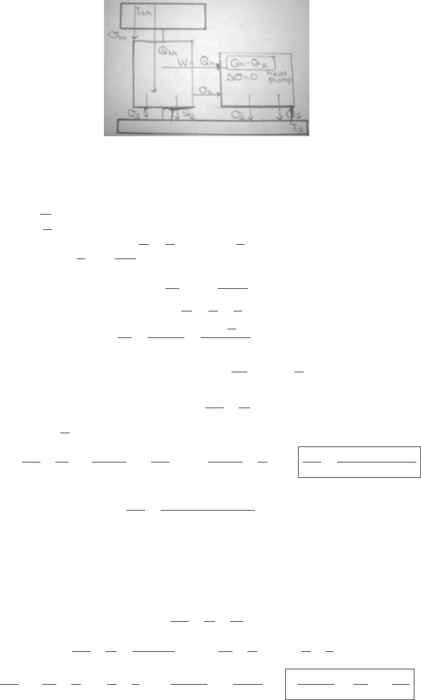
FIGURE 1. Problem 8.1(c)
Problems. Solution 1. Heat pump.
(a) For a heat pump,
input: σ
h
=
Q
h
τ
h
output: σ
l
=
Q
l
τ
l
Reversible condition: σ
h
= σ
l
=
Q
h
τ
h
=
Q
l
τ
l
so that Q
h
=
τ
h
τ
l
Q
l
.
Q
h
− Q
l
= Q
h
−
τ
l
τ
h
Q
h
=
τ
h
−τ
l
τ
h
Q
h
net heat inputted to pump heat.
Thus,
W
Q
h
= η
c
=
τ
h
− τ
l
τ
h
If heat pump is not reversible, σ
h
> σ
l
, so that
Q
h
τ
h
>
Q
l
τ
l
or
τ
l
τ
h
Q
h
> Q
l
,
W
Q
h
=
Q
h
− Q
l
Q
h
<
Q
h
−
τ
l
τ
h
Q
h
Q
h
= η
c, ideal
(b) Q
h
= electricity consumed by reversible heat pump.
Carnot engine: W = (τ
hh
− τ
l
)(σ
hh
− σ
l
), with σ
hh
=
Q
hh
τ
hh
, and σ
l
=
Q
l
τ
l
Condition that electricity consumed by reversible heat pump:
W = (τ
hh
− τ
l
)
Q
hh
τ
hh
−
Q
l
τ
l
= Q
h
Note we let σ
l
=
Q
l
τ
l
since both heat pump andCarnot engine are reversible.
=⇒
Q
hh
τ
hh
−
Q
h
τ
h
=
Q
h
τ
hh
− τ
l
=⇒
Q
hh
τ
hh
= Q
h
1
τ
hh
− τ
l
+
1
τ
h
=⇒
Q
hh
Q
h
=
τ
hh
(τ
h
+ τ
hh
− τ
l
)
τ
h
(τ
hh
− τ
l
)
For T
hh
= 600 K, T
h
= 300 K, T
l
= 270 K,
Q
hh
Q
h
=
600(300 + 600 − 270)
300(600 − 270)
= 3.82
(c) See Figure (1).
Solution 2. Absorption refrigerator.
(a) See Figure (2).
(b) Given τ
hh
> τ
h
,
by energy conservation: Q
hh
+ Q
l
− Q
h
= 0
reversible refrigerator: σ
hh
+ σ
l
− σ
h
= 0,
=⇒
Q
hh
τ
hh
+
Q
l
τ
l
−
Q
h
τ
h
= 0
Q
hh
τ
hh
+
Q
l
τ
l
=
Q
hh
+ Q
l
τ
h
or Q
hh
1
τ
hh
−
1
τ
h
= Q
l
1
τ
h
−
1
τ
l
Q
l
Q
hh
=
1
τ
hh
−
1
τ
h
/
1
τ
h
−
1
τ
l
=
τ
h
− τ
hh
τ
h
τ
hh
/
τ
l
− τ
h
τ
h
τ
l
=
τ
hh
− τ
h
τ
h
− τ
l
τ
l
τ
hh
=
Q
l
Q
hh
Note that Q
l
− Q
h
= Q
l
− (Q
hh
+ Q
l
) = −Q
hh
; we’ve removed Q
hh
heat from refrigerator’s inside.
31

FIGURE 2. Problem 8.2(a)
Solution 3. Photon Carnot engine. Recall, photons are relativistic: = pc. Recall p =
~
i
∇. =⇒
s
= pc = ~k
s
c =
n
s
π
L
~c.
Recalling that there are 2 polarization states for a photon in 3-dim. space,
U = (2)
1
8
(4π)
Z
∞
0
n
2
dn
nπ
L
~c
e
−
nπ
L
~c/τ
=
π
2
~c
L
Z
∞
0
n
3
dnexp
−π~c
Lτ
n
=
=
π
2
~c
L
{n
3
exp
−π~c
Lτ
n
Lτ
−π~c
∞
0
−
Z
∞
0
3n
2
exp
−π~c
Lτ
n
Lτ
−π~c
dn} =
=
π
2
~c
L
{(−1)
−Kτ
π~c
3
Z
∞
0
n
2
exp
−π~c
Lτ
n
dn} =
=
π
2
~c
L
{(−1)
−Lτ
π~c
3{n
2
exp
−π~c
Lτ
n
Lτ
−π~c
∞
0
−
Z
∞
0
2nexp
−π~c
Lτ
n
Lτ
−π~c
dn =
=
π
2
~c
L
(−1)
2
−Lτ
π~c
2
3(2)
Z
∞
0
nexp
−π~c
Lτ
n
Lτ
−π~c
dn =
=
π
2
~c
L
(−1)
3
−Lτ
π~c
3
3(2)(1)
Z
∞
0
exp
−π~c
Lτ
n
dn =
π
2
~c
L
(−1)
3
−Lτ
π~c
4
3(2)1
exp
−π~c
Lτ
n
∞
0
=
= 6
L
π
2
~c
3
τ
4
= 6
V
(π
2
~c)
3
τ
4
= U
To get the entropy, recall,
∂σ
∂U
V
=
1
τ
, and using this is usually the most direct way to obtain entropy.
=⇒ dσ =
Z
dU
τ
=
Z
6V
(π
2
~
2
c)
3
4τ
3
dτ
τ
=
6V
(π
2
~
2
c)
3
1
3
τ
3
=⇒ σ(τ ) =
8V τ
3
(π
2
~
2
c)
3
Consider
Isothermal expansion: Helmholtz free energy F is needed.
F = U − τσ =
6V
(π
2
~
2
c)
3
τ
4
− τ
8V τ
3
(π
2
~
2
c)
3
= −
2V τ
4
(π
2
~
2
c)
3
Then
p = −
∂F
∂V
τ, N
=
2τ
4
(π
2
~
2
c)
3
W
12
= p(V
2
− V
1
) =
2τ
4
h
(π
2
~
2
c)
3
(V
2
− V
1
)
σ
12
=
8τ
3
h
(π
2
~
2
c)
3
(V
2
− V
1
)
∆Q
12
=
τ
∆
σ =
8τ
4
h
(π
2
~
2
c)
3
(V
2
− V
1
)
Isentropic expansion: =⇒ V
2
τ
3
h
= V
3
τ
3
l
or V
3
= V
2
τ
h
τ
l
3
.
So for this isentropic process, V
2
τ
3
h
= V τ
3
,
U =
6V
(π
2
~
2
c)
3
V
2
τ
3
h
V
4/3
=
6(V
2
τ
3
h
)
4/3
(π
2
~
2
c)
3
V
−1/3
32

p =
−∂U
∂V
= −
6(V
2
τ
3
h
)
4/3
(π
2
~
2
c)
3
−1
3
V
−4/3
=
2(V
2
τ
3
h
)
4/3
(π
2
~
2
c)
3
V
−4/3
W
23
=
Z
pdV =
Z
2(V
2
τ
3
h
)
4/3
(π
2
~
2
c)
3
V
−4/3
dV =
2(V
2
τ
3
h
)
4/3
(π
2
~
2
c)
3
(−3V
−1/3
)
V
3
V
2
=
−6(V
2
τ
3
h
)
4/3
(π
2
~
2
c)
3
1
V
1/3
3
−
1
V
1/3
2
!
=
=
6V
2
τ
4
h
(π
2
~
2
c)
3
1 −
τ
l
τ
h
Isothermal compression: W
34
=
2τ
4
l
(π
2
~
2
c)
3
(V
4
− V
3
) =
2τ
3
h
τ
l
(π
2
~
2
c)
3
(V
1
− V
2
).
σ
34
=
8τ
3
l
(π
2
~c)
3
(V
4
− V
3
) =
8τ
3
h
(π
2
~c)
3
(V
1
− V
2
).
Isentropic compressiong: V
4
τ
3
l
= V
1
τ
3
h
or V
4
= V
1
τ
h
τ
l
3
.
W
41
=
6(V
4
τ
3
l
)
4/3
(π
2
~
2
c)
3
1
V
1/3
4
−
1
V
1/3
1
!
=
−6V
1
τ
4
h
(π
2
~
2
c)
3
1 −
τ
l
τ
h
∆W =
2τ
4
h
(π
2
~
2
c)
3
(V
2
−V
1
)+
6V
2
τ
4
h
(π
2
~
2
c)
3
1 −
τ
l
τ
h
+
2τ
3
h
τ
l
(π
2
~
2
c)
3
(V
1
−V
2
)+
−6V
1
τ
4
h
(π
2
~
2
c)
3
1 −
τ
l
τ
h
=
8τ
4
h
(V
2
− V
1
)
(π
2
~
2
c)
3
1 −
τ
l
τ
h
Q
h
=
8τ
4
h
(V
2
− V
1
)
(π
2
~c)
3
=⇒
∆W
Q
h
= 1 −
τ
l
τ
h
Solution 4. Heat engine-refrigerator cascade. Consider the heat engine as a Carnot cycle.
W + W
r
= (τ
h
− τ
l
)σ
h
where W
r
= work consumed by refrigerator.
σ
h
=
Q
h
τ
h
=
Q
l
τ
l
= σ
l
This must be true for any heat engine undergoing Carnot cycle; furthermore, we can say it’s the most efficient heat engine
possible.
reversible refrigerator: Q
L
+ W
r
= Q
H
, (by E-consv.)
σ
L
= σ
H
=
Q
L
τ
L
=
Q
H
τ
H
, (by reversible condition)
Note, Q
l
is energy transfer from heat engine to τ
l
reservoir. Q
L
is energy transfer from τ
l
reservoir to refrigerator. Q
L
≥ Q
l
,
otherwise, no cooling, no thermal energy extracted from τ
l
resevoir to lower its temperature. Q
L
= Q
l
at equilibrium; no
further cooling, τ
r
reached.
Note that τ
l
is given as the environmental temperature. Assume refrigerator throws out Q
H
heat into the environment.
→ τ
H
= τ
l
. Since Q
L
heat inputed into refrigerator from a τ
l
reservoir now lowered to τ
r
, τ
l
→ τ
r
.
W
r
=
τ
l
τ
r
Q
L
− Q
L
=
τ
l
τ
r
− 1
Q
L
since for a reversible refrigerator, σ
L
= σ
H
=
Q
L
τ
L
=
Q
H
τ
H
.
=⇒
W
Q
h
=
1 −
τ
r
τ
h
−
τ
l
τ
r
− 1
Q
L
Q
h
=
1 −
τ
r
τ
h
−
τ
l
τ
r
− 1
τ
r
τ
h
= 1 −
τ
l
τ
h
Combinations of reversible systems = reversible system.
Solution 5. Thermal pollution. Given
T
l
= 20
◦
C
T
h
= 500
◦
C
. Consider a Carnot cycle.
W = (τ
h
− τ
l
)σ
l
= (τ
h
− τ
l
)
Q
l
τ
l
=
τ
h
τ
l
− 1
Q
l
=
500
20
− 1
1500 M W = 36000MW
If improvements in hot-steam technology would permit raising T
h
by 100
◦
C,
W =
600
20
− 1
1500 M W = (29)(1500 MW ) = 43500 M W
There was a 17.2 % increase in output.
Solution 6. Room air conditioner.
33

(a)
W = (τ
h
− τ
l
)
Q
l
τ
l
=
τ
h
τ
l
− 1
Q
l
P =
τ
h
τ
l
− 1
dQ
l
dt
=
τ
h
τ
l
− 1
A(τ
h
− τ
l
) =⇒
P
A
τ
l
= (τ
h
− τ
l
)(τ
h
− τ
l
) = τ
2
h
− 2τ
h
τ
l
+ τ
2
l
=⇒ τ
2
l
− 2τ
h
τ
l
−
P
A
τ
l
+ τ
2
h
= 0
τ
l
= τ
h
+
P
2A
−
r
(τ
h
+
P
2A
)
2
− τ
2
h
(b) For T
l
= 17
◦
C = 290 K, T
h
= 310 K,
A =
P τ
l
(τ
h
− τ
l
)
2
=
(2 kW )(290 K)
(310 − 290)
2
=
580 × 10
3
W
400 K
= 1450
W
K
Solution 7. Light bulb in a refrigerator
Carnot refrigerator draws 100 W. For any Carnot cycle,
W = (τ
h
− τ
l
)
Q
l
τ
l
=
τ
h
τ
l
− 1
Q
l
=
1 −
τ
l
τ
h
Q
h
Carnot refrigerator expels Q
h
thermal energy to hot τ
h
environment and inputs Q
l
thermal energy from τ
l
reservoir.
Q
l
+ W = Q
h
Work W must be drawn by Carnot refrigerator to do work. Suppose Carnot cycle part of the refrigerator must input in heat
from light bulb to cool down its inside, i.e. consider Carnot refrigerator in equilibrium with light bulb, now inputting in heat
from light bulb Q
ext
, and drawing in work to expend out Q
h
thermal energy into the environment.
=⇒ Q
ext
= Q
l
˙
W =
˙
Q
l
in this case, so
τ
h
τ
l
− 1
Q
l
− Q
l
= 0 or
τ
h
τ
l
− 2
Q
l
= 0
=⇒ τ
l
=
τ
h
2
=
300 K
2
= 150 K
Solution 8. Geothermal energy.
Given ∆Q
h
= −MCdT
h
,
T
l
lower reservoir temperature stays constant. τ
h
decreasing, dτ
h
< 0.
∆W = (τ
h
− τ
l
)
∆Q
h
τ
h
=
1 −
τ
l
τ
h
(−MC)
dτ
h
k
B
=⇒ W = −
MC
k
B
(τ
h
− τ
l
ln τ
h
)|
τ
f
τ
i
= −
MC
k
B
τ
l
ln
τ
i
τ
f
− (τ
i
− τ
f
)
For M = 10
17
g, C = 1 J/g ·K, T
l
= 20
◦
C = 293 K, T
i
= 600
◦
C = 873 K, T
f
= 110
◦
C = 383 K
W = 2.486 ×10
19
J
Note that 10
14
kW h = 10
17
J
s
· h
3600 sec
1 h
= 3.6 × 10
20
J.
Solution 9. Cooling of nonmetallic solid to T = 0. Recall that C = aT
3
=
∂U
∂T
V
. Then dQ
l
= aT
3
l
dT
l
. Now dτ
l
< 0
since τ
l
decreasing.
For the refrigerator: Q
l
+ W = Q
h
.
dW = (τ
h
− τ
l
)
Q
l
τ
l
= −
τ
h
τ
l
− 1
(aτ
3
l
dτ
l
)
1
k
4
B
=
−a
k
4
B
τ
h
τ
l
− 1
τ
3
l
dτ
l
=
−a
k
4
B
(τ
h
τ
2
l
− τ
3
l
)dτ
l
W =
−a
k
4
B
τ
h
1
3
τ
3
l
−
1
4
τ
4
l
0
τ
h
=
aT
3
h
12k
B
= W
34

9. GIBBS FREE ENERGY AND CHEMICAL REACTIONS
Solution 1. Thermal expansion near absolute zero
(a)
∂G
∂τ
N, p
= −σ
∂
2
G
∂p∂τ
τ
= −
∂σ
∂p
τ
∂G
∂p
τ
= V
∂
2
G
∂τ ∂p
p
=
∂V
∂τ
p
=⇒
∂V
∂τ
p
= −
∂σ
∂p
τ
∂G
∂N
p
= µ
∂
2
G
∂p∂N
N
=
∂µ
∂p
N
∂G
∂p
τ
= V
∂
2
G
∂N∂p
p
=
∂V
∂N
p
=⇒
∂V
∂N
p
=
∂µ
∂p
N
∂
2
G
∂τ ∂N
N
=
∂µ
∂τ
N
∂
2
G
∂N∂τ
τ
= −
∂σ
∂N
τ
=⇒
∂µ
∂τ
N
= −
∂σ
∂N
τ
(b) α =
1
V
∂V
∂τ
p
=
−1
V
∂σ
∂p
τ
= 0 as τ → 0 since σ → constant as τ → 0 by third law of thermodynamics.
Solution 2. Thermal ionization of hydrogen.
(a) Given e + H
+
H, note that e + H
+
− H = 0. Recall
[e][H
+
]
[H]
= K(τ) =
Y
j
n
ν
j
Q
j
exp [−ν
j
F
j
(int)/τ]
where n
Q
=
Mτ
2π~
2
3/2
V .
For dissocation of H into e
−
+ H
+
choose zero of internal energy of each composite particle (here H) to concide
with energy of dissociated particles (here H
+
, e
−
) at rest; place energy of ground state of composite particle H at
−I, I is energy required in reaction to dissociate composite particle into its constituents and is taken to be positive,
i.e. the ionization energy.
K(τ) = (n
e
−
)
1
exp [−F
int
(e
−
)/τ] · (n
H
+
)
1
exp [−F
int
(H
+
)/τ](n
H
)
−1
exp (−(−1)(F
int
(H)/τ ))
Note that n
H
+
' n
H
. Let n
e
−
= n
Q
. Importantly, note
F
int
(e
−
) + F
int
(H
+
) − F
int
(H) = I
F
int
(H) is at a lower free energy than e
−
and H
+
.
=⇒ K(τ ) = n
Q
e
−I/τ
=⇒
[e][H
+
]
[H]
= n
Q
e
−I/τ
(b) By charge conservation, [e] = [H
+
], so that
[e] = [H]
1/2
n
1/2
Q
exp (−I/2τ)
Given [H] ' 10
23
cm
−3
, m
e
= 0.511 M eV /c
2
, T = 5000 K, I = 13.6 eV ionization energy,
[e] = (10
23
cm
−3
)
1/2
(2.92 × 10
10
1/cm
3/2
)
1/2
exp (−13.6 eV /2k
B
5000 K) = 1.3 × 10
15
cm
−3
Note that H(exc) and H are just two different states of atomic hydrogen. Their concentrations must therefore be
proportional to the probability of occurrence of these states, and the ratio of probabilities is the ratio of the respective
Boltzmann
[H(exc)]
[H]
=
p(H(exc))
p(H)
If
H(exc)
is the internal energy of the first excited state and
H
is the internal energy of the ground state of atomic
hydrogen, we are given that
H(exc)
−
H
=
3
4
I. We also need to take into account the fact that the first excited
electronic state of hydrogen is 4-fold degenerate i.e. one 2s-orbital and three 2p-orbitals.
1
Therefore,
[H(exc)]
[H]
=
p(H(exc))
p(H)
=
4e
−
H(exc)
/τ
e
−
H
/τ
= 4e
−3I/4τ
[H(exc)] = 4[H]e
−3I/4τ
= 2.092 × 10
13
cm
−3
1
(from solutions to Homework 8, Ph12c, Caltech, June 6, 2008, by Prabha Mandayam, Heywood Tam)
35

[e]
[H(exc)]
= 62
Solution 4. Biopolymer growth.
Recall that G(N, p, τ ) = N µ(p, τ ), since G was chosen to be an extensive quantity (it scales with size). For more than one
chemical species G =
P
j
N
j
µ
j
.
dF = 0 for equilibrium, for constant P, τ.
µ
j
= chemical potential of species j, µ
j
= (∂G/∂N
j
)
τ,p
.
Given
P
i
ν
j
A
j
, e.g. H
2
+ Cl
2
= 2HCl,
dG = (
P
j
ν
j
µ
j
)d
ˆ
N where dN
j
= ν
j
d
ˆ
N, dG = 0 →
P
j
ν
j
µ
j
= 0.
Recall the mass action law derivation: assume constituents act as ideal gases; µ
j
= τ(ln n
j
− ln c
j
), n
j
concentration of
species j; c
j
≡ n
Q
j
Z
j
(int).
X
j
ν
j
ln n
j
=
X
j
ν
j
ln c
j
=⇒
X
j
ln n
ν
j
j
=
X
j
ln c
ν
j
j
= ln
Y
j
n
ν
j
j
= ln K(τ)
Y
j
n
ν
j
j
= K(τ) mass action law
(a) By mass action law,
[ monomer][Nmer]
[(N+1)mer]
=
[1][N]
[N+1]
= K
N
.
[1][1]
[2]
= K
1
[1]
2
[2]
[1][2]
[3]
=
[1]
3
[3]
= K
1
K
2
[1]
j+1
[j + 1]
[1][j + 1]
[j + 2]
=
j
Y
l=1
K
l
K
j+1
=
[1]
j+2
[j + 2]
=
j+1
Y
l=1
K
l
=⇒ [N + 1] = [1]
N+1
/K
1
K
2
K
3
. . . K
N
(b) Recall that K(τ) =
Q
j
n
ν
j
Q
j
exp [−ν
j
F
j
(int)/τ]
K
N
=
n
Q
(N)n
Q
(1)
n
Q
(N + 1)
exp
−F
N
τ
−
F
1
τ
exp
F
N+1
τ
=
n
Q
(N)n
Q
(1)
n
Q
(N + 1)
exp
−(F
N
+ F
1
− F
N+1
)
τ
where n
Q
(N) =
M
N
τ
2π~
2
3/2
and M
N
is the mass of Nmer molecules, F
N
is the free energy of one Nmer molecule.
(c) Assume N 1 so n
Q
(N) ' n
Q
(N + 1). Assume [1] = 10
20
cm
−3
. Assume ∆F = F
N+1
− F
N
− F
1
= 0,
meaning zero free energy change in the basic reaction step. We’re given the molecular weight of the monomer to be
200.
We want
[N+1]
[N]
at room temperature. Now K
N
' n
Q
(1) =
M
1
τ
2π~
2
3/2
.
[1][N]
[N + 1]
= n
Q
(1) =
M
1
τ
2π~
2
3/2
or
[N + 1]
[N]
=
[1]
n
Q
(1)
=
2π~
2
M
1
τ
3/2
10
20
cm
−3
Note that
2π(6.582×10
−22
MeV ·s)
2
200(938MeV /c
2
)(0.8617×10
−4
eV/K)(298 K)
3×10
10
cm/s
1 c
2
3/2
= 0.3627 × 10
−27
cm.
=⇒
[N + 1]
[N]
= 3.627 × 10
−8
(d) We want the condition
1 <
[N + 1]
[N]
=
[1]
n
Q
(1)
exp
−∆F
τ
or ln
n
Q
(1)
[1]
<
−∆F
τ
=⇒ ∆F < τ ln
[1]
n
Q
(1)
= −0.44 eV
36

10. PHASE TRANSFORMATIONS
11. BINARY MIXTURES
12. CRYOGENICS
13. SEMICONDUCTOR STATISTICS
14. KINETIC THEORY
15. PROPAGATION
Heat Conduction Equation. nonrelativistic case:
Let manifold N = R ×M, with dimM = n.
Let J ∈ X(N ) = X(R × M) be a vector field in N.
Let
ρ ∈ C
∞
(N)
ρ = ρ(t, x) locally
be a smooth function on N.
Let J ∈ Ω
1
(N) be a 1-form on N that is isomorphic to J (Tangent-Cotangent isomorphism theorem), i.e.
J = J
[
J
i
= g
ij
J
j
with g
ij
being the metric on N (not just M!)
Note that as N = R ×M, g
0j
= δ
0j
The local form of J is the following:
J = ρ
∂
∂t
+ j
i
∂
∂x
i
i = 1 . . . n
So
J = J
i
dx
i
= g
ij
J
j
dx
i
= ρdt + j
k
dx
k
k = 1 . . . n
Thus
(21) J = ρdt + j
k
dx
k
k = 1 . . . n
Now do the Hodge star operator, resulting in a n-form
∗J ∈ Ω
n
(N)
and so
∗J = ρ ∗ dt + j
k
∗ dx
k
= ρvol
n
+ i
j
vol
n+1
as
ρ ∗ dt = ρ
√
g
n!
0
i
1
...i
n
dx
i
1
∧ ··· ∧ dx
i
n
i
1
. . . i
n
∈ {1 . . . n}
j
k
∗ dx
k
= g
kl
j
l
√
g
(n + 1)!
k
i
1
...i
n
dx
i
1
∧ ··· ∧ dx
i
n
= i
j
vol
n+1
so thus
∗J = ρvol
n
+ i
j
vol
n+1
Hence
(22) d ∗ J =
∂
∂t
(ρ
√
g)
1
√
g
vol
n+1
+
∂
∂x
k
(
√
gj
k
)
1
√
g
vol
n+1
= d(ρvol
n
) + di
j
vol
n+1
Special case:
∂
√
g
∂t
= 0
d ∗ J =
∂ρ
∂t
vol
n+1
+
∂
∂x
k
ln
√
g
j
k
vol
n+1
+
∂j
k
∂x
k
vol
n+1
= 0
=⇒
∂ρ
∂t
+
∂
∂x
k
ln
√
g
j
k
+
∂j
k
∂x
k
= 0
Special case: if
√
g constant,
∂ρ
∂t
+
∂j
k
∂x
k
= 0
Let j ≡ −Ddρ (j is a closed form on M ) where dρ =
∂ρ
∂x
i
dx
i
i = 1 . . . n, D constant
d ∗ J = dρvol
n
+ −Dd ∗ dρ = 0
37

For flat metric,
√
g constant,
∂ρ
∂t
= D
∂
2
ρ
(∂x
k
)
2
For relativistic case,
Consider manifold M, with dimension dimM = n + 1
J = ρ
∂
∂t
+ j
i
∂
∂x
i
Let J = J
[
. J
µ
= g
µν
J
ν
For special case of flat Minkowski space,
J = −ρdt + j
i
dx
i
∗J = −ρ ∗ dt + j
i
∗ dx
i
− ρ
√
g
(n + 1)!
0
i
1
...i
n
dx
i
1
∧ ··· ∧ dx
i
n
+ j
i
√
g
(n + 1)!
i
µ
1
...µ
n
dx
µ
1
∧ ··· ∧ dx
µ
n
d ∗ J = −
∂(ρ
√
g)
∂t
1
√
g
vol
n+1
+
∂(j
i
√
g)
∂x
i
1
√
g
vol
n+1
= 0
=⇒ −
∂(ρ
√
g)
∂t
+
∂(j
i
√
g)
∂x
i
= 0
Fick law (14.19) for particle flux density, j = −D
n
dn where
D
n
particle diffusivity constant
n particle concentration
J = ndt + j
thermal conductivity; homogeneous medium
b
C heat capacity per unit volume. j
u
= −Kdτ
J =
b
Cτdt + j
u
(23)
b
C
∂τ
∂t
+
∂(j
u
)
k
∂x
k
= 0 (5)
(24)
∂τ
∂t
= D
τ
∂
2
τ
(∂x
k
)
2
D
τ
≡ K/
b
C (6)
Propagation of Sound Waves in Gases. pressure associated with sound wave
(25) δp = δp
0
exp [i(kx −ωt)] (27)
Suppose ideal gas:
(26) pV = N τ or p = ρτ/M (28)
Consider “solid ball” or “billiard ball” particle (extended particle, not pt. particle, but no internal structure)
ρ =
NM
V
Force on particle
F =
dP
dt
=
d
dt
Z
ρvol
n
u =
M
V
Z
L
∂
∂t
+u
u =
M
V
Z
∂u
∂t
+ [u, u]
Suppose [u, u] = 0 (certainly for flat spaces; what about for curved spaces? [u, u] 6= 0? Possibly? I don’t know. EY:
20150317
(27) dU + pdV = τdσ
define fractional deviations s, θ
(28)
ρ = ρ
0
(1 + s)
τ = τ
0
(1 + θ)
(5)
where ρ
0
, τ
0
are density and temperature in absence of sound wave.
assume u, s, θ have form of traveling exp [i(kx − ωt)]
38

ωu −
kτ
M
s −
kτ
M
θ = 0 (39)(29)
ωs − ku = 0 (40)(30)
τ
b
C
V
θ − ps = 0 or
b
C
V
θ − ns = 0 (41)(31)
ωu =
kτ
M
1 +
n
b
C
V
s
ω =
kτ
M
1 +
n
b
C
V
k
ω
So
(32) ω =
γτ
M
1/2
k (42)
γ =
b
C
V
+ n
b
C
V
=
b
C
p
b
C
V
v
s
=
∂ω
∂k
=
γτ
M
1/2
Problems. Problem 1. Fourier analysis of pulse
t = 0
(33) θ(x, 0) = δ(x) =
1
2π
Z
∞
−∞
dk exp (ikx) (58)
(34) θ(x, t) =
1
2π
Z
∞
−∞
dk exp [i(kx −ωt)] (59)
Given a dispersion relation at this form:
(35) Dk
2
= iω (10)
(36) θ(x, t) =
1
2π
Z
∞
−∞
dk exp [ikx −Dk
2
t] (60)
and so, doing the Gaussian integral,
(37) θ(x, t) =
1
√
4πDt
exp
−x
2
4Dt
(14)
Problem Diffusion in two and three dimensions.
(a)
∂θ
2
∂t
= −
θ
2
t
+
r
2
4
θ
2
Dt
2
∂
2
θ
2
(∂x
i
)
2
= −
1
2
θ
2
Dt
−
1
2
θ
2
Dt
+
1
4
θ
2
D
2
t
2
(x
2
+ y
2
)
=⇒
∂θ
2
∂t
= D
∂
2
θ
2
(∂x
i
)
2
(b)
(c)
39
REFERENCES
[1] Charles Kittel, Herbert Kroemer, Thermal Physics, W. H. Freeman; Second Edition edition, 1980. ISBN-13: 978-0716710882
[2] Bernard F. Schutz, Geometrical Methods of Mathematical Physics, Cambridge University Press, 1980. ISBN-13: 978-0521298872
[3] Paul Bamberg and Shlomo Sternberg, A Course in Mathematics for students of physics: 2, Cambridge University Press, 1990.
[4] T. Frankel, The Geometry of Physics, Cambridge University Press, Second Edition, 2004.
There is a Third Edition of T. Frankel’s The Geometry of Physics [4], but I don’t have the funds to purchase the book (about
$ 71 US dollars, with sales tax). It would be nice to have the hardcopy text to see new updates and to use for research, as the
second edition allowed me to formulate fluid mechanics and elasticity in a covariant manner. Please help me out and donate
at ernestyalumni.tilt.com or at subscription based Patreon, patreon.com/ernestyalumni.
E-mail address: [email protected]
URL: http://ernestyalumni.wordpress.com
40
