Monetary Policy Report, July 13, 2018

Board of Governors of the Federal Reserve System

For use at 11:00 a.m., EDT

July 13, 2018

Monetary Policy rePort

July 13, 2018

Letter of transmittaL

B  G  

F R S

Washington, D.C., July 13, 2018

T P   S

T S   H  R

The Board of Governors is pleased to submit its Monetary Policy Report pursuant to

section 2B of the Federal Reserve Act.

Sincerely,

Jerome H. Powell, Chairman

Adopted effective January24, 2012; as amended effective January30, 2018

The Federal Open Market Committee (FOMC) is rmly committed to fullling its statutory

mandate from the Congress of promoting maximum employment, stable prices, and moderate

long-term interest rates. The Committee seeks to explain its monetary policy decisions to the public

as clearly as possible. Such clarity facilitates well-informed decisionmaking by households and

businesses, reduces economic and nancial uncertainty, increases the eectiveness of monetary

policy, and enhances transparency and accountability, which are essential in a democratic society.

Ination, employment, and long-term interest rates uctuate over time in response to economic and

nancial disturbances. Moreover, monetary policy actions tend to inuence economic activity and

prices with a lag. Therefore, the Committee’s policy decisions reect its longer-run goals, its medium-

term outlook, and its assessments of the balance of risks, including risks to the nancial system that

could impede the attainment of the Committee’s goals.

The ination rate over the longer run is primarily determined by monetary policy, and hence the

Committee has the ability to specify a longer-run goal for ination. The Committee rearms its

judgment that ination at the rate of 2percent, as measured by the annual change in the price

index for personal consumption expenditures, is most consistent over the longer run with the

Federal Reserve’s statutory mandate. The Committee would be concerned if ination were running

persistently above or below this objective. Communicating this symmetric ination goal clearly to the

public helps keep longer-term ination expectations rmly anchored, thereby fostering price stability

and moderate long-term interest rates and enhancing the Committee’s ability to promote maximum

employment in the face of signicant economic disturbances. The maximum level of employment

is largely determined by nonmonetary factors that aect the structure and dynamics of the labor

market. These factors may change over time and may not be directly measurable. Consequently,

it would not be appropriate to specify a xed goal for employment; rather, the Committee’s policy

decisions must be informed by assessments of the maximum level of employment, recognizing that

such assessments are necessarily uncertain and subject to revision. The Committee considers a

wide range of indicators in making these assessments. Information about Committee participants’

estimates of the longer-run normal rates of output growth and unemployment is published four

times per year in the FOMC’s Summary of Economic Projections. For example, in the most

recent projections, the median of FOMC participants’ estimates of the longer-run normal rate of

unemployment was 4.6percent.

In setting monetary policy, the Committee seeks to mitigate deviations of ination from its

longer-run goal and deviations of employment from the Committee’s assessments of its maximum

level. These objectives are generally complementary. However, under circumstances in which the

Committee judges that the objectives are not complementary, it follows a balanced approach in

promoting them, taking into account the magnitude of the deviations and the potentially dierent

time horizons over which employment and ination are projected to return to levels judged

consistent with its mandate.

The Committee intends to rearm these principles and to make adjustments as appropriate at its

annual organizational meeting each January.

statement on Longer-run goaLs and monetary PoLicy strategy

contents

Note: This report reects information that was publicly available as of noon EDT on July12, 2018.

Unless otherwise stated, the time series in the gures extend through, for daily data, July11, 2018; for monthly data,

June2018; and, for quarterly data, 2018:Q1. In bar charts, except as noted, the change for a given period is measured to

its nal quarter from the nal quarter of the preceding period.

For gures 16 and 34, note that the S&P 500 Index and the Dow Jones Bank Index are products of S&P Dow Jones Indices LLC and/or its afliates and

Redistribution, reproduction, and/or photocopying in whole or in part are prohibited without written permission of S&P Dow Jones Indices LLC. For more

information on any of S&P Dow Jones Indices LLC’s indices please visit www.spdji.com. S&P® is a registered trademark of Standard & Poor’s Financial

Services LLC, and Dow Jones® is a registered trademark of Dow Jones Trademark Holdings LLC. Neither S&P Dow Jones Indices LLC, Dow Jones Trademark

Holdings LLC, their afliates nor their third party licensors make any representation or warranty, express or implied, as to the ability of any index to

accurately represent the asset class or market sector that it purports to represent, and neither S&P Dow Jones Indices LLC, Dow Jones Trademark Holdings

LLC, their afliates nor their third party licensors shall have any liability for any errors, omissions, or interruptions of any index or the data included therein.

For gure A in the box “Interest on Reserves and Its Importance for Monetary Policy,” note that neither DTCC Solutions LLC nor any of its afliates shall

be responsible for any errors or omissions in any DTCC data included in this publication, regardless of the cause and, in no event, shall DTCC or any of

its afliates be liable for any direct, indirect, special or consequential damages, costs, expenses, legal fees, or losses (including lost income or lost prot,

trading losses and opportunity costs) in connection with this publication.

Summary ..................................................1

Economic and Financial Developments ......................................... 1

Monetary Policy

........................................................... 2

Special Topics

............................................................. 2

Part 1: Recent Economic and Financial Developments ................ 5

Domestic Developments. . . . . . . . . . . . . . . . . . . . . . . . . . . . . . . . . . . . . . . . . . . . . . . . . . . . . 5

Financial Developments

.................................................... 23

International Developments

................................................. 30

Part 2: Monetary Policy ....................................... 35

Part 3: Summary of Economic Projections ......................... 47

The Outlook for Economic Activity ............................................ 48

The Outlook for Ination

................................................... 50

Appropriate Monetary Policy

................................................ 51

Uncertainty and Risks

...................................................... 51

Abbreviations ..............................................63

List of Boxes

The Labor Force Participation Rate for Prime-Age Individuals ......................... 8

The Recent Rise in Oil Prices

................................................ 16

Developments Related to Financial Stability

..................................... 26

Complexities of Monetary Policy Rules

......................................... 37

Interest on Reserves and Its Importance for Monetary Policy

......................... 44

Forecast Uncertainty

....................................................... 62

summary

Economic activity increased at a solid pace

over the rst half of 2018, and the labor

market has continued to strengthen. Ination

has moved up, and in May, the most recent

period for which data are available, ination

measured on a 12-month basis was a little

above the Federal Open Market Committee’s

(FOMC) longer-run objective of 2percent,

boosted by a sizable increase in energy prices.

In this economic environment, the Committee

judged that current and prospective economic

conditions called for a further gradual removal

of monetary policy accommodation. In line

with that judgment, the FOMC raised the

target for the federal funds rate twice in the

rst half of 2018, bringing it to a range of

1¾to 2percent.

Economic and Financial

Developments

The labor market. The labor market has

continued to strengthen. Over the rst

six months of 2018, payrolls increased an

average of 215,000 per month, which is

somewhat above the average pace of 180,000

per month in 2017 and is considerably faster

than what is needed, on average, to provide

jobs for new entrants into the labor force.

The unemployment rate edged down from

4.1percent in December to 4.0percent in June,

which is about ½percentage point below the

median of FOMC participants’ estimates of

its longer-run normal level. Other measures

of labor utilization were consistent with a

tight labor market. However, hourly labor

compensation growth has been moderate,

likely held down in part by the weak pace of

productivity growth in recent years.

Ination. Consumer price ination, as

measured by the 12-month percentage change

in the price index for personal consumption

expenditures, moved up from a little below

the FOMC’s objective of 2percent at the end

of last year to 2.3percent in May, boosted by

a sizable increase in consumer energy prices.

The 12-month measure of ination that

excludes food and energy items (so-called core

ination), which historically has been a better

indicator of where overall ination will be in

the future than the total gure, was 2percent

in May. This reading was ½percentage point

above where it had been 12 months earlier, as

the unusually low readings from last year were

not repeated. Measures of longer-run ination

expectations have been generally stable.

Economic growth. Real gross domestic product

(GDP) is reported to have increased at an

annual rate of 2percent in the rst quarter

of 2018, and recent indicators suggest that

economic growth stepped up in the second

quarter. Gains in consumer spending slowed

early in the year, but they rebounded in

the spring, supported by strong job gains,

recent and past increases in household

wealth, favorable consumer sentiment, and

higher disposable income due in part to the

implementation of the Tax Cuts and Jobs Act.

Business investment growth has remained

robust, and indexes of business sentiment have

been strong. Foreign economic growth has

remained solid, and net exports had a roughly

neutral eect on real U.S. GDP growth in the

rst quarter. However, activity in the housing

market has leveled o this year.

Financial conditions. Domestic nancial

conditions for businesses and households

have generally continued to support economic

growth. After rising steadily through 2017,

broad measures of equity prices are modestly

higher, on balance, from their levels at the end

of last year amid some bouts of heightened

volatility in nancial markets. While long-

term Treasury yields, mortgage rates, and

yields on corporate bonds have risen so far

this year, longer-term interest rates remain

low by historical standards, and corporate

bond issuance has continued at a moderate

pace. Moreover, most types of consumer loans

2 SUMMARY

remained widely available for households with

strong creditworthiness, and credit provided by

commercial banks continued to expand. The

foreign exchange value of the U.S. dollar has

appreciated somewhat against the currencies

of our trading partners this year, but it

remains below its level at the start of 2017.

Foreign nancial conditions remain generally

supportive of growth despite recent increases

in nancial stress in several emerging market

economies.

Financial stability. The U.S. nancial system

remains substantially more resilient than

during the decade before the nancial crisis.

Asset valuations continue to be elevated

despite declines since the end of 2017 in the

forward price-to-earnings ratio of equities and

the prices of corporate bonds. In the private

nonnancial sector, borrowing among highly

levered and lower-rated businesses remains

elevated, although the ratio of household

debt to disposable income continues to be

moderate. Vulnerabilities stemming from

leverage in the nancial sector remain low,

reecting in part strong capital positions

at banks, whereas some measures of hedge

fund leverage have increased. Vulnerabilities

associated with maturity and liquidity

transformation among banks, insurance

companies, money market mutual funds,

and asset managers remain below levels that

generally prevailed before2008.

Monetary Policy

Interest rate policy. Over the rst half of 2018,

the FOMC has continued to gradually increase

the target range for the federal funds rate.

Specically, the Committee decided to raise

the target range for the federal funds rate at

its meetings in March and June, bringing it

to the current range of 1¾ to 2percent. The

decisions to increase the target range for the

federal funds rate reected the economy’s

continued progress toward the Committee’s

objectives of maximum employment and price

stability. Even with these policy rate increases,

the stance of monetary policy remains

accommodative, thereby supporting strong

labor market conditions and a sustained return

to 2percent ination.

The FOMC expects that further gradual

increases in the target range for the federal

funds rate will be consistent with a sustained

expansion of economic activity, strong labor

market conditions, and ination near the

Committee’s symmetric 2percent objective

over the medium term. Consistent with this

outlook, in the most recent Summary of

Economic Projections (SEP), which was

compiled at the time of the June FOMC

meeting, the median of participants’

assessments for the appropriate level for

the federal funds rate rises gradually over

the period from 2018 to 2020 and stands

somewhat above the median projection for

its longer-run level by the end of 2019 and

through 2020. (The June SEP is presented

in Part 3 of this report.) However, as the

Committee has continued to emphasize, the

timing and size of future adjustments to the

target range for the federal funds rate will

depend on the Committee’s assessment of

realized and expected economic conditions

relative to its maximum-employment objective

and its symmetric 2percent ination objective.

Balance sheet policy. The FOMC has

continued to implement the balance sheet

normalization program described in the

Addendum to the Policy Normalization

Principles and Plans that the Committee issued

about a year ago. Specically, the FOMC has

been reducing its holdings of Treasury and

agency securities by decreasing, in a gradual

and predictable manner, the reinvestment

of principal payments it receives from these

securities.

Special Topics

Prime-age labor force participation. Labor

force participation rates (LFPRs) for men and

women between 25 and 54years old—that is,

the share of these individuals either working

or actively seeking work—trended lower

MONETARY POLICY REPORT: JULY 2018 3

between 2000 and 2013. Those trends likely

reect numerous factors, including a long-run

decline in the demand for workers with lower

levels of education and an increase in the

share of the population with some form of

disability. By contrast, the prime-age LFPR

has increased notably since 2013, and the

share of nonparticipants who report wanting

a job remains above pre-recession levels. Thus,

some continuation of the recent increase in

the prime-age LFPR may be possible if labor

demand remains strong. (See the box “The

Labor Force Participation Rate for Prime-Age

Individuals” in Part 1.)

Oil prices. Oil prices have climbed rapidly

over the past year, reecting both supply and

demand factors. Although higher oil prices

are likely to restrain household consumption

in the United States, much of the negative

eect on GDP from lower consumer spending

is likely to be oset by increased production

and investment in the growing U.S. oil sector.

Consequently, higher oil prices now imply

much less of a net overall drag on the economy

than they did in the past, although they will

continue to have important distributional

eects. The negative eect of upward moves

in oil prices should get smaller still as U.S. oil

production grows and net oil imports decline

further. (See the box “The Recent Rise in Oil

Prices” in Part 1.)

Monetary policy rules. Monetary policymakers

consider a wide range of information on

current economic conditions and the outlook

when deciding on a policy stance they deem

most likely to foster the FOMC’s statutory

mandate of maximum employment and stable

prices. They also routinely consult monetary

policy rules that connect prescriptions for the

policy interest rate with variables associated

with the dual mandate. The use of such rules

requires, among other considerations, careful

judgments about the choice and measurement

of the inputs into the rules such as estimates

of the neutral interest rate, which are highly

uncertain. (See the box “Complexities of

Monetary Policy Rules” in Part 2.)

Interest on reserves. The payment of interest

on reserves—balances held by banks in

their accounts at the Federal Reserve—is an

essential tool for implementing monetary

policy because it helps anchor the federal

funds rate within the FOMC’s target range.

This tool has permitted the FOMC to achieve

a gradual increase in the federal funds rate in

combination with a gradual reduction in the

Fed’s securities holdings and in the supply

of reserve balances. The FOMC judged that

removing monetary policy accommodation

through rst raising the federal funds rate

and then beginning to shrink the balance

sheet would best contribute to achieving and

maintaining maximum employment and

price stability without causing dislocations in

nancial markets or institutions that could put

the economic expansion at risk. (See the box

“Interest on Reserves and Its Importance for

Monetary Policy” in Part 2.)

Domestic Developments

The labor market strengthened further

during the rst half of the year . . .

Labor market conditions have continued to

strengthen so far in 2018. According to the

Bureau of Labor Statistics (BLS), gains in

total nonfarm payroll employment averaged

215,000 per month over the rst half of the

year. That pace is up from the average monthly

pace of job gains in 2017 and is considerably

faster than what is needed to provide jobs for

new entrants into the labor force (gure1).

Indeed, the unemployment rate edged down

from 4.1percent in December to 4.0percent

in June (gure2). This rate is below all

Federal Open Market Committee (FOMC)

participants’ estimates of its longer-run

normal level and is about ½percentage point

below the median of those estimates.

The

unemployment rate in June is close to the lows

last reached in 2000.

The labor force participation rate (LFPR),

which is the share of individuals aged 16

and older who are either working or actively

looking for work, was 62.9percent in June

and has changed little, on net, since late

2013 (gure3). The aging of the population

is an important contributor to a downward

trend in the overall participation rate. In

particular, members of the baby-boom

cohort are increasingly moving into their

retirement years, a time when labor force

participation is typically low. Indeed, the

share of the civilian population aged 65

and over in the United States climbed from

16percent in 2000 to 19percent in 2017 and

is projected to rise to 24percent by 2026.

Given this trend, the at trajectory of the

1. Monthly job gains in the range of 130,000 to

160,000 are consistent with an unchanged unemployment

rate and an unchanged labor force participation rate.

2. See the Summary of Economic Projections in Part3

of this report.

Part 1

recent economic and financiaL deveLoPments

Total nonfarm

800

600

400

200

400

Thousands of jobs

2018201720162015201420132012201120102009

1. Net change in payroll employment

3-month moving averages

Private

OURCE

: Bureau of Labor Statistics via Haver Analytics.

6 PART 1: RECENT ECONOMIC AND FINANCIAL DEVELOPMENTS

LFPR during the past few years is consistent

with strengthening labor market conditions.

Similarly, the LFPR for individuals between

25 and 54years old—which is much less

sensitive to population aging—has been rising

for the past several years. (The box “The

Labor Force Participation Rate for Prime-

Age Individuals” examines the prospects for

further increases in participation for these

individuals.) The employment-to-population

ratio for individuals 16 and over—the share

of the total population who are working—

was 60.4percent in June and has been

gradually increasing since 2011, reecting the

combination of the declining unemployment

rate and the at LFPR.

Other indicators are also consistent with

a strong labor market. As reported in the

Job Openings and Labor Turnover Survey

(JOLTS), the rate of job openings has

remained quite elevated.

The rate of quits has

3. Indeed, the number of job openings now about

matches the number of unemployed individuals.

Employment-to-population ratio

Prime-age labor force

participation rate

Percent

20182015201220092006

3. Labor force participation rates and

employment-to-population ratio

Percent

Labor force participation rate

NOTE: The data are monthly. The prime-age labor force participation

rate

is a percentage of the population aged 25 to 54. The labor force

participation

rate and the employment-to-population ratio are percentages of the

population

aged 16 and over.

SOURCE: Bureau of Labor Statistics via Haver Analytics.

U-5

U-4

U-6

Percent

2018201620142012201020082006

2. Measures of labor underutilization

Monthly

Unemployment rate

OTE

: Unemployment rate measures total unemployed as a percentage of the labor force. U-4 measures total unemployed plus discouraged workers, as

percentage of the labor force plus discouraged workers. Discouraged workers are a subset of marginally attached workers who are not currently looking for work

because they believe no jobs are available for them. U-5 measures total unemployed plus all marginally attached to the labor force, as a percentage of the

labor

force plus persons marginally attached to the labor force. Marginally attached workers are not in the labor force, want and are

available for work, and have looked

for a job in the past 12 months. U-6 measures total unemployed plus all marginally attached workers plus total employed part time for economic reasons, as

percentage of the labor force plus all marginally attached workers. The shaded bar indicates a period of business recession as defined by the National Bureau

Economic Research.

OURCE

: Bureau of Labor Statistics via Haver Analytics.

MONETARY POLICY REPORT: JULY 2018 7

stayed high in the JOLTS, an indication that

workers are able to successfully switch jobs

when they wish to. In addition, the JOLTS

layo rate has been low, and the number of

people ling initial claims for unemployment

insurance benets has remained near its

lowest level in decades. Other survey evidence

indicates that households perceive jobs as

plentiful and that businesses see vacancies as

hard to ll. Another indicator, the share of

workers who are working part time but would

prefer to be employed full time—which is part

of the U-6 measure of labor underutilization

from the BLS—fell further in the rst six

months of the year and now stands close to its

pre-recession level (as shown in gure2).

. . . and unemployment rates have fallen

for all major demographic groups

The continued decline in the unemployment

rate has been reected in the experiences of

multiple racial and ethnic groups (gure4).

The unemployment rates for blacks or

African Americans and Hispanics tend to

rise considerably more than rates for whites

and Asians during recessions but decline

Black or African American

Asian

Hispanic or Latino

Percent

2018201620142012201020082006

4. Unemployment rate by race and ethnicity

Monthly

White

OTE: Unemployment rate measures total unemployed as a percentage of the labor force. Persons whose ethnicity is identified as Hispanic or Latino may be of

any race. The shaded bar indicates a period of business recession as defined by the National Bureau of Economic Research.

OURCE: Bureau of Labor Statistics via Haver Analytics.

8 PART 1: RECENT ECONOMIC AND FINANCIAL DEVELOPMENTS

increases in automation, such as the use of robotics,

and various aspects of globalization have spurred

the elimination of some types of jobs—in particular,

some manufacturing jobs that have historically been

held by workers without a college education—and

emerging jobs may require a different set of skills. These

developments may have led some workers to become

discouraged over the lack of suitable job opportunities

and drop out of the labor force.

The rising share of

college-educated workers, which may partly reect

individuals responding over time to the declining

demand for jobs that require less education, has likely

prevented even steeper declines in the prime-age LFPR,

as better-educated workers have higher LFPRs and

may be more adaptable to unforeseen disruptions in

particular jobs or industries.

Another potential factor may be that an increasing

share of the prime-age population has some difculty

working because of physical or mental disabilities.

For example, gure C shows that about 5percent of

both prime-age men and women report that they are

out of the labor force and do not want a job due to

disability or illness; those shares have trended higher

over the past several decades. Other research suggests

that increased opioid use may be associated with a

lower prime-age LFPR, although it is unclear how

much of the decline in the prime-age LFPR can be

directly explained by opioid use or whether increases

The overall labor force participation rate (LFPR) has

generally been trending lower since 2000, and while

the aging of the baby-boom generation into retirement

ages provides an important reason for that decline,

it is not the only reason. Another contributing factor,

as shown in gureA, is that the LFPRs of prime-age

men and women (those between 25 and 54years

old) trended lower through 2013 even though prime-

age LFPRs are largely unaffected by the aging of

the population: The prime-age male LFPR has been

declining for six decades, and the prime-age female

LFPR has drifted lower since 2000 after a multidecade

increase. Nevertheless, prime-age LFPRs have moved

up notably and consistently since 2013, as improving

labor market conditions have drawn some individuals

back into the labor force and encouraged others not to

leave. These recent increases in the prime-age LFPR,

in the context of the longer-run trend decline, raise the

question of how much additional scope there is for

further increases in prime-age labor force participation.

To gauge whether further increases are possible, a

useful starting point is understanding the factors behind

the longer-run decline in the prime-age LFPR, as these

factors may limit additional increases if they continue

to exert some downward pressure. One factor may

be a secular decline in the demand for workers with

lower levels of education. Indeed, as shown in gureB,

the long-run declines in prime-age LFPR are much

larger among adults without a college degree than

among college-educated adults. Research suggests that

The Labor Force Participation Rate for Prime-Age Individuals

Men

Percent

201820132008200319981993198819831978

A. Prime-age labor force participation rates

Monthly

Women

OTE: The data are seasonally adjusted. The shaded bars indicate

periods

business recession as defined by the National Bureau of

Economic

Research.

OURCE: Bureau of Labor Statistics.

1. For evidence on displacement from technological

changes, see David H. Autor, David Dorn, and Gordon H.

Hanson (2015), “Untangling Trade and Technology: Evidence

from Local Labor Markets,” Economic Journal, vol.125 (May),

pp. 621–46; Daron Acemoglu and Pascual Restrepo (2017),

“Robots and Jobs: Evidence from U.S. Labor Markets,” NBER

Working Paper Series 23285 (Cambridge, Mass.: National

Bureau of Economic Research, March), www.nber.org/

papers/w23285; and Daron Acemoglu and Pascual Restrepo

(2018), “Articial Intelligence, Automation, and Work,” NBER

Working Paper Series 24196 (Cambridge, Mass.: National

Bureau of Economic Research, January), www.nber.org/

papers/w24196. For evidence on globalization—in particular,

import competition since the 2000s—see David H. Autor,

David Dorn, and Gordon H. Hanson (2013), “The China

Syndrome: Local Labor Market Effects of Import Competition

in the United States,” American Economic Review, vol. 103

(October), pp. 2121–68. A discussion of these and other

explanations is also provided in Katharine G. Abraham and

Melissa S. Kearney (2018), “Explaining the Decline in the U.S.

Employment-to-Population Ratio: A Review of the Evidence,”

NBER Working Paper Series 24333 (Cambridge, Mass.:

National Bureau of Economic Research, February), www.nber.

org/papers/w24333.

(continued)

MONETARY POLICY REPORT: JULY 2018 9

responsibilities as women participate in the workforce

in greater numbers. For some—especially those for

whom childcare costs are not a major concern—not

participating in the labor force may represent an

unconstrained choice to care for other members of their

families. For others, however, this decision may reect

a lack of affordable childcare.

Additionally, the share of the population—

particularly black men—with a history of incarceration

has increased over time. Individuals who have

previously been incarcerated often have trouble nding

work, in part because many employers choose not to

hire people with such a background and likely also

in part because incarceration prevents people from

accumulating work experience and developing skills

valuable to employers. Discrimination could also help

explain the lack of participation for some minority

groups, as they recognize that such discrimination

limits their job opportunities.

International comparisons may help clarify the

importance of some of those factors. Since 1990, the

in opioid use are an indirect result of poor employment

opportunities.

Caregiving responsibilities play an important role in

explaining why LFPRs for prime-age women are lower

than for men, and they may play an increasing role in

explaining declining prime-age LFPRs for men as well.

As shown in gure C, roughly 15percent of prime-

age women report being out of the labor force for

caregiving reasons—by far the largest reason for prime-

age women to report not wanting a job—but this share

has been fairly at over time. In contrast, while a much

smaller fraction of men are out of the labor force for

caregiving reasons, that share has trended up in recent

decades, likely reecting some shift in household

2. Evidence that opioid use could be signicant for

understanding the declining LFPR is provided by Alan B.

Krueger (2017), “Where Have All the Workers Gone? An

Inquiry into the Decline of the U.S. Labor Force Participation

Rate,” Brookings Papers on Economic Activity, Fall, pp. 1–82,

https://www.brookings.edu/wp-content/uploads/2018/02/

kruegertextfa17bpea.pdf, while little relationship between

opioid prescriptions and employment at the county level is

found in Janet Currie, Jonas Y. Jin, and Molly Schnell (2018),

“U.S. Employment and Opioids: Is There a Connection?”

NBER Working Paper Series 24440 (Cambridge, Mass.:

National Bureau of Economic Research, March), www.nber.

org/papers/w24440. Some evidence on whether the opioid

epidemic varies with local economic conditions is provided

by Jeff Larrimore, Alex Durante, Kimberly Kreiss, Ellen Merry,

Women

Men

B. Prime-age labor force participation rates by education

N: The data are seasonally adjusted 12-month moving averages and extend through May 2018. The shaded bars indicate

periods of business recession as dened by the National Bureau of Economic Research.

S: U.S. Census Bureau, Current Population Survey.

Monthly PercentMonthly Percent

Bachelor's degree

High school degree or less 82

201820132008200319981993198819831978

Some college

Bachelor's degree

High school degree or less

201820132008200319981993198819831978

Some college

Christina Park, and Claudia Sahm (2018), “Shedding Light on

Our Economic and Financial Lives,” FEDS Notes, https://www.

federalreserve.gov/econres/notes/feds-notes/shedding-light-on-

our-economic-and-nancial-lives-20180522.htm.

(continued on next page)

10 PART 1: RECENT ECONOMIC AND FINANCIAL DEVELOPMENTS

self-report as wanting a job (despite not having actively

searched for a job recently) has been declining since

2010, that share for men remains between ¼ and

½percentage point above its 2007 level and earlier

expansion peaks. Furthermore, prime-age men and

women who had previously reported being out of the

labor force and not wanting a job due to disability or

illness have been entering the labor force at increasing

rates in recent years.

Looking forward, how can policymakers support

additional improvements in the prime-age LFPR?

Favorable labor market conditions can likely help,

and monetary policy can therefore play a role through

supporting strong cyclical conditions as part of its

maximum-employment objective. However, structural

factors (in contrast with cyclical ones) are also

important to address; policies to address such factors

are beyond the scope of monetary policy.

prime-age LFPR in the United States has declined

considerably for both men and women relative to other

advanced countries. Some factors, like automation and

globalization, have affected all advanced economies to

some degree and for some time, yet diverging long-run

trends in prime-age labor force participation have still

occurred. Research suggests that part of the relative

decline in the United States is explained by differential

changes in work-family policies across countries.

Other parts of the divergence may be explained by

other policies, including policies designed toward

keeping those affected by automation and globalization

attached to the labor force, or other factors—such as

incarceration or opioid use—that differ across those

countries.

Although many of the factors behind the

multidecade decline in the prime-age LFPR may

persist, some continuation of the increases in the LFPR

over the past few years nevertheless seems possible,

especially if labor market conditions remain favorable.

Indeed, as shown in gure C, although the share of

nonparticipating prime-age men and women who

3. For recent trends on prime-age LFPRs in the United

States compared with other developed countries, see

Organisation for Economic Co-operation and Development

(2018), OECD Economic Surveys: United States 2018 (Paris:

OECD Publishing), dx.doi.org/10.1787/eco_surveys-usa-2018-

en. For a description of policy differences across countries

Disabled

Caregiving

Wants job

2018201420102006200219981994

Other, does not want job

Disabled

Caregiving

Wants job

2018201420102006200219981994

Other, does not want job

PercentMonthly Monthly Percent

N: The data are seasonally adjusted 12-month moving averages and extend through May 2018. The shaded bars indicate

periods of business recession as dened by the National Bureau of Economic Research.

S: U.S. Census Bureau, Current Population Survey.

Women

Men

C. Prime-age nonparticipation by reason

The Labor Force Participation Rate (continued)

and how this may affect differences in LFPR, see International

Monetary Fund (2018), “Labor Force Participation in Advanced

Economies: Drivers and Prospects,” chapter 2 in World

Economic Outlook: Cyclical Upswing, Structural Change

(Washington: IMF, April), pp.71–128. For evidence on how

work-family policies may affect prime-age LFPRs in the United

States relative to other OECD countries, see Francine D. Blau

and LawrenceM. Kahn (2013), “Female Labor Supply: Why

Is the United States Falling Behind?” American Economic

Review, vol. 103 (May), pp. 251–56.

MONETARY POLICY REPORT: JULY 2018 11

more rapidly during expansions. Indeed,

the declines in the unemployment rates for

blacks and Hispanics have been particularly

striking, and the rates have recently been at

or near their lowest readings since these series

began in the early 1970s. Although dierences

in unemployment rates across ethnic and

racial groups have narrowed in recent years,

they remain substantial and similar to pre-

recession levels. The rise in LFPRs for prime-

age individuals over the past few years has

also been evident in each of these racial and

ethnic groups, with increases again particularly

notable for African Americans. Even so, the

LFPR for whites remains higher than that for

the other groups (gure5).

Increases in labor compensation have

been moderate . . .

Despite the strong labor market, the available

indicators generally suggest that increases

in hourly labor compensation have been

moderate. Compensation per hour in the

business sector—a broad-based measure

of wages, salaries, and benets that is quite

volatile—rose 2¾percent over the four

quarters ending in 2018:Q1, slightly more than

the average annual increase over the preceding

seven or so years (gure6). The employment

cost index—a less volatile measure of both

wages and the cost to employers of providing

benets—likewise was 2¾percent higher in

the rst quarter of 2018 relative to its year-

earlier level; this increase was ½percentage

point faster than its gain a year earlier. Among

measures that do not account for benets,

average hourly earnings rose 2¾percent in

June relative to 12months earlier, a gain in

line with the average increase in the preceding

few years. According to the Federal Reserve

Bank of Atlanta, the median 12-month wage

4. The lower levels of labor force participation for

these other groups dier importantly by sex. For African

Americans, men have a lower participation rate relative

to white men, while the participation rate for African

American women is as high as that of white women. By

contrast, the lower LFPRs for Hispanics and Asians

reect lower participation among women.

Employment cost index

Atlanta Fed's

Wage Growth Tracker

Average hourly earnings

Percent change from year earlier

20182016201420122010

6. Measures of change in hourly compensation

Compensation per hour,

business sector

OTE

: Business-sector compensation is on a 4-quarter percentage

change

basis. For the employment cost index, change is over the 12 months ending in

the last month of each quarter; for average hourly earnings, change is from

months earlier; for the Atlanta Fed's Wage Growth Tracker, the data

are

shown as a 3-month moving average of the 12-month percent change

and

extend through May 2018.

OURCE

: Bureau of Labor Statistics via Haver Analytics; Federal

Reserve

Bank of Atlanta, Wage Growth Tracker.

Black or African American

Asian

Hispanic or Latino

Percent

2018201620142012201020082006

5. Prime-age labor force participation rate by race and

ethnicity

Monthly

White

OTE

: The prime-age labor force participation rate is a percentage of the

population aged 25 to 54. Persons whose ethnicity is identified as Hispanic or

Latino may be of any race. The data are seasonally adjusted by Board staff

and are 3-month moving averages. The shaded bar indicates a period of

business recession as defined by the National Bureau of Economic Research.

OURCE

: Bureau of Labor Statistics.

12 PART 1: RECENT ECONOMIC AND FINANCIAL DEVELOPMENTS

growth of individuals reporting to the Current

Population Survey increased about 3¼percent

in May, also similar to its readings from the

past few years.

. . . and likely have been restrained by

slow growth of labor productivity

Those moderate rates of compensation

gains likely reect the osetting inuences

of a strong labor market and persistently

weak productivity growth. Since 2008, labor

productivity has increased only a little more

than 1percent per year, on average, well below

the average pace from 1996 through 2007 of

2.8percent and also below the average gain in

the 1974–95 period of 1.6percent (gure7).

The weakness in productivity growth may

be partly attributable to the sharp pullback

in capital investment during the most recent

recession and the relatively slow recovery

that followed. However, considerable debate

remains about the reasons for the recent

slowdown in productivity growth and whether

it will persist.

Price ination has picked up from the

low readings in 2017

In 2017, ination remained below the FOMC’s

longer-run objective of 2percent. Partly

because the softness in some price categories

appeared idiosyncratic, Federal Reserve

policymakers expected ination to move

higher in 2018.

This expectation appears to be

5. The Atlanta Fed’s measure diers from others in

that it measures the wage growth only of workers who

were employed both in the current survey month and

12months earlier.

6. The box “Productivity Developments in the

Advanced Economies” in the July2017 Monetary

Policy Report provides more information. See Board

of Governors of the Federal Reserve System (2017),

Monetary Policy Report (Washington: Board of

Governors, July), pp. 12–13, https://www.federalreserve.

gov/monetarypolicy/2017-07-mpr-part1.htm.

7. Additional details can be found in the June2017

Summary of Economic Projections, an addendum to the

minutes of the June2017 FOMC meeting. See Board

of Governors of the Federal Reserve System (2017),

“Minutes of the Federal Open Market Committee,

Percent, annual rate

7. Change in business-sector output per hour

1948–

1974–

1996–

2000

2001–

2008–

present

NOTE

: Changes are measured from Q4 of the year immediately

preceding

the period through Q4 of the final year of the period. The final period

measured from 2007:Q4 through 2018:Q1.

SOURCE

: Bureau of Labor Statistics via Haver Analytics.

MONETARY POLICY REPORT: JULY 2018 13

on track so far. Consumer price ination, as

measured by the 12-month percentage change

in the price index for personal consumption

expenditures (PCE), moved up to 2.3percent

in May (gure8). Core PCE ination, which

excludes consumer food and energy prices that

are often quite volatile and typically provides

a better indication than the total measure of

where overall ination will be in the future,

was 2percent over the 12months ending in

May—0.5percentage point higher than it

had been one year earlier. The total measure

exceeded core ination because of a sizable

increase in consumer energy prices. In

contrast, food price ination has continued to

be low by historical standards—data through

May show the PCE price index for food and

beverages having increased less than ½percent

over the past year.

The higher readings in both total and core

ination relative to a year earlier reect faster

price increases for a wide range of goods and

services this year and the dropping out of the

12-month calculation of the steep one-month

decline in the price index for wireless telephone

services in March last year. The 12-month

change in the trimmed mean PCE price

index—an alternative indicator of underlying

ination produced by the Federal Reserve

Bank of Dallas that may be less sensitive

than the core index to idiosyncratic price

movements—slowed by less than core ination

over 2017 and has also increased a bit less

this year. This index rose 1.8percent over the

12months ending in May, up a touch from the

increase over the same period last year.

June13–14, 2017,” press release, July5, https://

www.federalreserve.gov/newsevents/pressreleases/

monetary20170705a.htm.

8. The trimmed mean index excludes whatever prices

showed the largest increases or decreases in a given

month; for example, the sharp decline in prices for

wireless telephone services in March2017 was excluded

from this index.

Excluding food

and energy

Trimmed mean

1.0

1.5

2.0

2.5

3.0

12-month percent change

20182017201620152014201320122011

8. Change in the price index for personal consumption

expenditures

Monthly

Total

NOTE

: The data extend through May 2018; changes are from one year

earlier.

SOURCE: For trimmed mean, Federal Reserve Bank of Dallas; for all else,

Bureau of Economic Analysis; all via Haver Analytics.

14 PART 1: RECENT ECONOMIC AND FINANCIAL DEVELOPMENTS

Oil prices have surged amid supply

concerns . . .

As noted, the faster pace of total ination

this year relative to core ination reects a

substantial rise in consumer energy prices.

Retail gasoline prices this year were driven

higher by a rise in oil prices. The spot price of

Brent crude oil rose from about $65 per barrel

in December to around $75per barrel in early

July (gure9). Although that increase took

place against a backdrop of continued strength

in global demand, supply concerns have

become more prevalent in recent months. (For

a discussion of the reasons behind the oil price

increases along with a review of the eects of

oil prices on U.S. economic growth, see the

box “The Recent Rise in Oil Prices.”)

. . . while prices of imports other than

energy have also increased

Nonfuel import prices rose sharply in early

2018, partly reecting the pass-through

of earlier increases in commodity prices

(gure10). In particular, metals prices posted

sizable gains late last year due to strong

global demand but have retreated somewhat

in recent weeks.

Survey-based measures of ination

expectations have been stable . . .

Expectations of ination likely inuence actual

ination by aecting wage- and price-setting

decisions. Survey-based measures of ination

expectations at medium- and longer-term

horizons have remained generally stable so

far this year. In the Survey of Professional

Forecasters conducted by the Federal Reserve

Bank of Philadelphia, the median expectation

for the annual rate of increase in the PCE

price index over the next 10years has been

around 2percent for the past several years

(gure11). In the University of Michigan

Surveys of Consumers, the median value

for ination expectations over the next 5 to

10years has been about 2½percent since

the end of 2016, though this level is about

¼percentage point lower than had prevailed

through 2014. In contrast, in the Survey of

Consumer Expectations conducted by the

Nonfuel import prices

100

102

July 2014 = 100

100

110

120

2018201720162015201420132012

10. Nonfuel import prices and industrial metals indexes

July 2014 = 100

Industrial metals

OTE

: The data for nonfuel import prices are monthly and extend through

May

2018. The data for industrial metals are a monthly average of daily data

and extend through June 29, 2018.

SOURCE

: For nonfuel import prices, Bureau of Labor Statistics; for

industrial

metals, S&P GSCI Industrial Metals Spot Index via Haver

Analytics.

Spot price

100

110

120

130

Dollars per barrel

2013 2014 2015 2016 2017 2018

9. Brent spot and futures prices

Weekly

24-month-ahead

futures contracts

OTE: The data are weekly averages of daily data and extend

through

July 11, 2018.

OURCE: ICE Brent Futures via Bloomberg.

MONETARY POLICY REPORT: JULY 2018 15

Federal Reserve Bank of New York, the

median of respondents’ expected ination rate

three years hence has been moving up recently

and is currently at the top of the range it has

occupied over the past couple of years.

. . . while market-based measures of

ination compensation have largely

moved sideways this year

Ination expectations can also be gauged

by market-based measures of ination

compensation. However, the inference

is not straightforward, because market-

based measures can be importantly aected

by changes in premiums that provide

compensation for bearing ination and

liquidity risks. Measures of longer-term

ination compensation—derived either from

dierences between yields on nominal Treasury

securities and those on comparable-maturity

Treasury Ination-Protected Securities

(TIPS) or from ination swaps—have moved

sideways for the most part this year after

having returned to levels seen in early 2017

(gure12).

The TIPS-based measure of

5-to-10-year-forward ination compensation

and the analogous measure of ination swaps

are now about 2percent and 2½percent,

respectively, with both measures below the

ranges that persisted for most of the 10years

before the start of the notable declines in

mid-2014.

9. Ination compensation implied by the TIPS

breakeven ination rate is based on the dierence, at

comparable maturities, between yields on nominal

Treasury securities and yields on TIPS, which are indexed

to the total consumer price index (CPI). Ination swaps

are contracts in which one party makes payments of

certain xed nominal amounts in exchange for cash

ows that are indexed to cumulative CPI ination over

some horizon. Focusing on ination compensation 5 to

10years ahead is useful, particularly for monetary policy,

because such forward measures encompass market

participants’ views about where ination will settle in the

long term after developments inuencing ination in the

short term have run their course.

10. As these measures are based on CPI ination,

one should probably subtract about ¼ to ½percentage

point—the average dierential with PCE ination over

the past two decades—to infer ination compensation on

a PCE basis.

Michigan survey expectations

for next 5 to 10 years

Percent

2018201620142012201020082006

SPF expectations

for next 10 years

11. Median inflation expectations

NOTE

: The Michigan survey data are monthly. The SPF data for

inflation

expectations for personal consumption expenditures are quarterly and

extend

from 2007:Q1 through 2018:Q2.

OURCE: University of Michigan Surveys of Consumers; Federal

Reserve

Bank of Philadelphia, Survey of Professional Forecasters (SPF).

Inflation swaps

1.0

1.5

2.0

2.5

3.0

3.5

Percent

20182016201420122010

12. 5-to-10-year-forward inflation compensation

Weekly

TIPS breakeven rates

OTE:The data are weekly averages of daily data and extend

through

July 6, 2018. TIPS is Treasury Inflation-Protected Securities.

SOURCE: Federal Reserve Bank of New York; Barclays; Federal

Reserve

Board staff estimates.

16 PART 1: RECENT ECONOMIC AND FINANCIAL DEVELOPMENTS

the country’s economic and political crisis. Prices also

increased after President Trump announced on May8

that the United States was withdrawing from the Iran

nuclear deal and that sanctions against Iranian oil

exports would be reinstated.

The pattern of spot and futures prices indicates

that market participants generally anticipate that oil

prices will decline slowly over the next few years, in

part reecting an expectation that supply, including

U.S. shale oil production, will grow to meet demand.

In addition, the higher prices put pressure on OPEC’s

November2016 agreement with certain non-OPEC

countries to restrain production. A stated aim of the

agreement was to reduce the glut in global inventories,

and, in recent months, inventory levels have fallen

rapidly toward long-run averages. In response to both

lower inventories and higher prices, OPEC leaders

slightly relaxed the production agreement in June this

Oil prices have increased more than 50percent

over the past year, with the spot price of Brent crude

oil rising from a bit below $50per barrel to around

$75per barrel (gureA). For much of the period,

further-dated futures prices remained relatively stable,

in the neighborhood of $55per barrel; however, since

February, futures prices have moved up appreciably,

reaching over $70per barrel.

Both supply and demand factors have contributed

to the oil price increase. In particular, the broad-based

improvement in the outlook for the global economy

was a key driver of the price increase in the second

half of 2017. In recent months, supply concerns have

become more prevalent, affecting both spot and further-

dated futures prices. Despite sharply rising U.S. oil

production, markets have been attuned to escalating

conict between Saudi Arabia and Iran as well as the

precipitous decline in Venezuelan oil production amid

The Recent Rise in Oil Prices

Spot price

Dollars per barrel

Jan. Mar. May July Sept. Nov. Jan. Mar. May July

20182017

A. Brent spot and futures prices

Daily

December 2019 futures price

OURCE

: ICE Brent Futures via Bloomberg.

(continued)

MONETARY POLICY REPORT: JULY 2018 17

power abroad than in the past, as much of the negative

effect on GDP from lower household consumption

is likely to be offset by increased production and

investment in the growing U.S. oil sector. On net, the

drag on GDP from higher oil prices is likely a small

fraction of what it was a decade ago and should get

smaller still if U.S. oil production continues to grow

as projected—gure C—and the net oil import share

shrinks toward zero.

Indeed, if U.S. oil trade moves fully into balance,

the offsetting effects of a change in the relative price of

oil might be expected to net out within the domestic

economy. However, even if the United States is no

longer a net oil importer, to the extent that higher

oil prices cause credit-constrained consumers to cut

spending by more than oil producers expand their

investment, this redistribution of purchasing power

could still have negative effects on overall GDP.

year, reducing some of the upward pressure on prices.

That said, futures prices have not returned to their early

2018 levels, implying that market participants expect

some of the recent increase in prices to be long lasting.

What is the expected effect of the recent rise in oil

prices on the U.S. economy? To begin with, higher oil

prices are likely to restrain household consumption.

In particular, the increase in oil prices since last year

is estimated to have translated into a roughly $300

increase in annual expenditures on gasoline for the

average household, from about $2,100 to $2,400.

However, as U.S. oil production has grown rapidly

over the past decade, the ratio of net U.S. oil imports

to U.S. gross domestic product (GDP) has declined

substantially (gure B). As a result, higher oil prices

now imply much less of a redistribution of purchasing

1.0

1.5

2.0

2.5

3.0

3.5

Percent of nominal GDP

2019201720152013201120092007200520032001

B. Net oil import share

Quarterly

NOTE:

The data extending through 2018:Q1 are quarterly averages of daily

oil

futures prices, quarterly averages of monthly oil imports and exports,

and

quarterly

GDP. The data from 2018:Q2 through 2019:Q4 are

projections

based

on quarterly averages of monthly oil futures prices, quarterly

averages

of monthly oil imports and exports, and quarterly GDP.

SOURCE: Department of Energy via Haver Analytics; ICE Brent Futures

via

Bloomberg; Bureau of Economic Analysis; staff calculations.

Million barrels per day

201920182017201620152014

C. U.S. crude oil production

Quarterly

NOTE: The data are quarterly averages of monthly data. The data

extend

through 2018:Q2. Data from 2018:Q3 through 2019:Q4 are projections.

OURCE

: Department of Energy via Haver Analytics.

18 PART 1: RECENT ECONOMIC AND FINANCIAL DEVELOPMENTS

Real gross domestic product growth

slowed in the rst quarter, but spending

by households appears to have picked up

in recent months

After having expanded at an annual rate of

3percent in the second half of 2017, real gross

domestic product (GDP) is now reported to

have increased 2percent in the rst quarter of

this year (gure13). The step-down in growth

during the rst quarter was largely attributable

to a sharp slowing in the growth of consumer

spending that appears transitory, and gains in

GDP appear to have rebounded in the second

quarter. Meanwhile, business investment has

remained strong, and net exports had little

eect on output growth in the rst quarter. On

balance, over the rst half of this year, overall

economic activity appears to have expanded at

a solid pace.

The economic expansion continues to be

supported by favorable consumer and business

sentiment, past increases in household

wealth, solid economic growth abroad, and

accommodative domestic nancial conditions,

including moderate borrowing costs and easy

access to credit for many households and

businesses.

Gains in income and wealth continue to

support consumer spending . . .

Following exceptionally strong growth in the

fourth quarter of 2017, consumer spending

in the rst quarter of this year was tepid,

rising at an annual rate of 0.9percent. The

slowdown in growth was evident in outlays

for motor vehicles and in retail sales more

generally; moreover, unseasonably warm

weather depressed spending on energy services.

However, consumer spending picked up in

more recent months as retail sales rmed, and

PCE in April and May rose at an annual rate

of 2¼percent relative to the average over the

rst quarter (gure14).

Real disposable personal income (DPI), a

measure of after-tax income adjusted for

ination, has increased at a solid annual rate

of about 3percent so far this year. Real DPI

Percent, annual rate

2018201720162015201420132012

14. Change in real personal consumption expenditures

and disposable personal income

NOTE

: The values for 2018:H1 are the annualized May/Q4 changes.

SOURCE

: Bureau of Economic Analysis via Haver Analytics.

Personal consumption expenditures

Disposable personal income

PercentMonthly

2018201620142012201020082006

15. Personal saving rate

NOTE

: Data are through May 2018.

OURCE

:Bureau of Economic Analysis via Haver Analytics.

Percent, annual rate

20182017201620152014201320122011

13. Change in real gross domestic product and gross

domestic income

SOURCE: Bureau of Economic Analysis via Haver Analytics.

Gross domestic product

Gross domestic income

MONETARY POLICY REPORT: JULY 2018 19

has been supported by the reduction in income

taxes owing to the implementation of the

Tax Cuts and Jobs Act (TCJA) as well as the

continued strength in the labor market. With

consumer spending rising just a little less than

the gains in disposable income so far this year,

the personal saving rate has edged up after

having fallen for the past two years (gure15).

Ongoing gains in household net worth likely

have also supported consumer spending.

House prices, which are of particular

importance for the balance sheet positions of

a large set of households, have been increasing

at an average annual pace of about 6percent in

recent years (gure16).

Although U.S. equity

prices have posted modest gains, on net, so far

this year, this attening followed several years

of sizable gains. Buoyed by the cumulative

increases in home and equity prices, aggregate

household net worth was 6.8times household

income in the rst quarter, down just slightly

from its ratio in the fourth quarter—the

highest-ever reading for that ratio, which dates

back to 1947 (gure17).

. . . and borrowing conditions for

consumers remain generally favorable . . .

Financing conditions for consumers are

generally favorable and remain supportive

of growth in household spending. However,

banks have continued to tighten standards

for credit cards and auto loans for borrowers

with low credit scores, possibly in response

to some upward moves in the delinquency

rates of those borrowers. Mortgage credit has

remained readily available for households with

solid credit proles. For borrowers with low

credit scores, mortgage nancing conditions

have eased somewhat further but remain tight

overall. In this environment, consumer credit

continued to increase in the rst few months

of 2018, though the rate of increase moderated

some from its robust pace in the previous year

(gure18).

11. For the majority of households, home equity

makes up the largest share of their wealth.

CoreLogic

price index

S&P/Case-Shiller

national index

Percent change from year earlier

201820162014201220102008

16. Prices of existing single-family houses

Monthly

Zillow index

OTE

: The data for the S&P/Case-Shiller index extend through April

2018.

The

data for the Zillow index and the CoreLogic index extend through

May

2018.

OURCE: CoreLogic Home Price Index; Zillow; S&P/Case-Shiller

U.S.

National Home Price Index. The S&P/Case-Shiller Index is a product of S&P

Dow

Jones Indices LLC and/or its affiliates. (For Dow Jones

Indices

licensing information, see the note on the Contents page.)

5.0

5.5

6.0

6.5

7.0

Ratio

2018201520122009200620032000

17. Wealth-to-income ratio

Quarterly

NOTE

: The series is the ratio of household net worth to disposable personal

income.

SOURCE: For net worth, Federal Reserve Board, Statistical Release

Z.1,

“Financial

Accounts of the United States”; for income, Bureau of

Economic

Analysis via Haver Analytics.

600

400

200

400

600

800

1,000

Billions of dollars, annual rate

201820162014201220102008

18. Changes in household debt

Sum

NOTE

: Changes are calculated from year-end to year-end except

2018

changes, which are calculated from 2017:Q4 to 2018:Q1.

OURCE: Federal Reserve Board, Statistical Release Z.1,

“Financial

Accounts of the United States.”

Mortgages

Consumer credit

20 PART 1: RECENT ECONOMIC AND FINANCIAL DEVELOPMENTS

Billions of dollars, monthly rate

201820162014201220102008

21. Selected components of net debt financing for

nonfinancial businesses

Sum

OURCE

: Federal Reserve Board, Statistical Release Z.1,

“Financial

Accounts of the United States.”

Commercial paper

Bonds

Bank loans

Percent, annual rate

201820172016201520142013201220112010

20. Change in real private nonresidential fixed investment

OURCE

: Bureau of Economic Analysis via Haver Analytics.

Structures

Equipment and intangible capital

. . . while consumer condence remains

strong

Consumers have remained upbeat. So far this

year, the Michigan survey index of consumer

sentiment has been near its highest level

since 2000, likely reecting rising income, job

gains, and low ination (gure19). Indeed,

households’ expectations for real income

changes over the next year or two now stand

above levels preceding the previous recession.

Business investment has continued

to rebound . . .

Investment spending by businesses has

continued to increase so far this year, with

notable gains for spending, both on equipment

and intangibles and on nonresidential

structures (gure20). Within structures,

the rise in oil prices propelled another steep

ramp-up in investment in drilling and mining

structures—albeit not yet back to the levels

recorded from 2012 to 2014—while investment

in nonresidential structures outside of the

energy sector picked up after declining in

2017. Forward-looking indicators of business

investment spending remain favorable on

balance. Business sentiment and the prot

expectations of industry analysts have been

positive overall, while new orders of capital

goods have advanced on net this year.

. . . while corporate nancing conditions

have remained accommodative

Aggregate ows of credit to large nonnancial

rms remained strong in the rst quarter,

supported in part by relatively low interest

rates and accommodative nancing conditions

(gure21). The gross issuance of corporate

bonds stayed robust during the rst half of

2018, while yields on both investment- and

speculative-grade corporate bonds moved

up notably but remained low by historical

standards (gure22). Despite strong growth in

business investment, outstanding commercial

and industrial (C&I) loans on banks’ books

rose only modestly in the rst quarter,

although their pace of expansion in more

recent months has strengthened on average. In

Consumer sentiment

100

110

Index

2018201620142012201020082006

Diffusion index

19. Indexes of consumer sentiment and income expectations

Real income expectations

OTE

: The consumer sentiment data are monthly and are indexed to 100 in

1966. The real income expectations data are calculated as the net percentage

of survey respondents expecting family income to go up more than prices

during the next year or two plus 100 and are shown as a three-month moving

average.

OURCE

: University of Michigan Surveys of Consumers.

MONETARY POLICY REPORT: JULY 2018 21

April, respondents to the Senior Loan Ocer

Opinion Survey on Bank Lending Practices,

or SLOOS, reported that demand for C&I

loans weakened in the rst quarter even as

lending standards and terms on such loans

eased.

Respondents attributed this decline in

demand in part to rms drawing on internally

generated funds or using alternative sources of

nancing. Meanwhile, growth in commercial

real estate loans has moderated some but

remains strong. In addition, nancing

conditions for small businesses appear to

have remained generally accommodative, with

lending standards little changed at most banks

and with most rms reporting that they are

able to obtain credit. Although small business

credit growth has been subdued, survey data

suggest this sluggishness is largely due to

continued weak demand for credit by small

businesses.

But activity in the housing sector has

leveled off

Residential investment, which rose a modest

2½percent in 2017, appears to have largely

moved sideways over the rst ve months of

the year. The slowing in residential investment

likely is partly a result of higher mortgage

interest rates. Although these rates are still

low by historical standards, they have moved

up and are near their highest levels in seven

years (gure23). In addition, higher lumber

prices and tight supplies of skilled labor

and developed lots reportedly have been

restraining home construction. While starts

of both single-family and multifamily housing

units rose in the fourth quarter, single-family

starts have been little changed, on net, since

then, whereas multifamily starts continued

to climb earlier this year before attening

out (gure24). Meanwhile, over the rst ve

months of this year, new home sales have

held at around the rate of late last year, but

sales of existing homes have eased somewhat

(gure25). Despite the continued increases

in house prices, the pace of construction has

12. The SLOOS is available on the Board’s website at

https://www.federalreserve.gov/data/sloos/sloos.htm.

Double-A

High-yield

Percentage points

2000 2003 2006 2009 2012 2015 2018

22. Corporate bond yields, by securities rating

Daily

Triple-B

OTE: The yields shown are yields on 10-year bonds.

OURCE

: ICE Bank of America Merrill Lynch Indices, used

with

permission.

Mortgage rates

105

125

145

165

185

205

Index

20182016201420122010

23. Mortgage rates and housing affordability

Percent

Housing affordability index

OTE: The housing affordability index data are monthly

through

April

2018, and the mortgage rate data are weekly through July 5, 2018.

an index value of 100, a median-income family has exactly enough income to

qualify

for a median-priced home mortgage. Housing affordability

seasonally adjusted by Board staff.

SOURCE

: For housing affordability index, National Association of

Realtors;

for mortgage rates, Freddie Mac Primary Mortgage Market Survey.

Multifamily starts

Single-family permits

1.2

1.6

2.0

Millions of units, annual rate

2018201620142012201020082006

24. Private housing starts and permits

Monthly

Single-family starts

OTE

: The data extend through May 2018.

SOURCE

: U.S. Census Bureau via Haver Analytics.

22 PART 1: RECENT ECONOMIC AND FINANCIAL DEVELOPMENTS

not kept up with demand. As a result, the

months’ supply of inventories of homes for

sale has remained at a relatively low level, and

the aggregate vacancy rate stands at the lowest

level since 2003.

Net exports had a neutral effect on GDP

growth in the rst quarter

After being a small drag on U.S. real GDP

growth last year, net exports had a neutral

eect on growth in the rst quarter. Real

U.S. exports increased about 3½percent at

an annual rate, as exports of automobiles

and consumer goods remained robust. Real

import growth slowed sharply following

a surge late last year (gure26). Nominal

trade data through May suggest that export

growth picked up in the second quarter, led

by agricultural exports, while import growth

was tepid. All told, the available data suggest

that the nominal trade decit likely narrowed

relative to GDP in the second quarter

(gure27).

Fiscal policy became more expansionary

this year . . .

Federal scal policy will likely provide a

moderate boost to GDP growth this year. The

individual and corporate tax cuts in the TCJA

should lead to increased private consumption

and investment, while the Bipartisan Budget

Act of 2018 (BBA) enables increased federal

spending on goods and services. As the eects

of the BBA had yet to show through, federal

government purchases posted only a modest

gain in the rst quarter (gure28).

After narrowing signicantly for several years,

the federal unied decit widened from about

2½percent of GDP in scal year 2015 to

3½percent in scal 2017, and it is on pace

to move up further in scal 2018. Although

expenditures as a share of GDP in 2017

were relatively stable at 21percent, receipts

moved lower to roughly 17percent of GDP

and have remained at about the same level so

far this year (gure29). The ratio of federal

Percent, annual rate

2018201720162015201420132012

26. Change in real imports and exports of goods

and services

OURCE

: Bureau of Economic Analysis via Haver Analytics.

Imports

Exports

Current account

Percent of nominal GDP

201820162014201220102008200620042002

27. U.S. trade and current account balances

Quarterly

Trade

OTE: GDP is gross domestic product.

OURCE

: Bureau of Economic Analysis via Haver Analytics.

Existing home sales

1.0

1.2

1.4

1.6

Millions, annual rate

3.0

3.5

4.0

4.5

5.0

5.5

6.0

6.5

7.0

7.5

2018201620142012201020082006

25. New and existing home sales

Millions, annual rate

New home sales

OTE: Data are monthly and extend through May 2018. New home

sales

includes only single-family sales. Existing home sales includes single-family,

condo, townhome, and co-op sales.

OURCE: For new home sales, U.S. Census Bureau; for existing

home

sales, National Association of Realtors; all via Haver Analytics.

MONETARY POLICY REPORT: JULY 2018 23

debt held by the public to nominal GDP was

76½percent at the end of scal 2017 and is

quite elevated relative to historical norms

(gure30).

. . . and the scal position of most state

and local governments is stable

The scal position of most state and local

governments remains stable, although there is a

range of experiences across these governments

and some states are still struggling. After

several years of slow growth, revenue gains of

state governments have strengthened notably

as sales and income tax collections have picked

up over the past few quarters. In addition,

house price gains have continued to push up

property tax revenues at the local level. But

expenditures by state and local governments

have been restrained. Employment growth

in this sector has been moderate, while real

outlays for construction by these governments

have largely been moving sideways at a

relatively low level.

Financial Developments

The expected path of the federal funds

rate has moved up

Market-based measures of the path of the

federal funds rate continue to suggest that

market participants expect further gradual

increases in the federal funds rate. Relative

to the end of last year, the expected policy

rate path has moved up, boosted in part by

investors’ perception of a strengthening in

the domestic economic outlook (gure31).

In particular, the policy path moved higher

in response to incoming economic data so far

this year, especially the employment reports,

which were seen as supporting expectations for

a solid pace of growth in domestic economic

activity. In addition, investors reportedly

interpreted FOMC communications in the rst

half of 2018 as signaling an upbeat economic

outlook and as reinforcing expectations for

further gradual removal of monetary policy

accommodation.

Percent, annual rate

2018201720162015201420132012201120102009

28. Change in real government expenditures on

consumption and investment

SOURCE

: Bureau of Economic Analysis.

Federal

State and local

Expenditures

Percent of nominal GDPPercent of nominal GDP

20182015201220092006200320001997

Annual

29. Federal receipts and expenditures

Receipts

OTE

: Through 2017, receipts and expenditures are for fiscal years

(October

to September); gross domestic product (GDP) is for the four

quarters

ending in Q3. For 2018, receipts and expenditures are for the

months ending in May; GDP is the average of 2017:Q4 and 2018:Q1.

Receipts and expenditures are on a unified-budget basis.

OURCE

: Office of Management and Budget via Haver Analytics.

Percent of nominal GDP

Quarterly

30. Federal government debt held by the public

1968 1978 1988 1998 2008 2018

OTE: The data for gross domestic product (GDP) are at an annual rate.

Federal

debt held by the public equals federal debt less Treasury securities

held in federal employee defined benefit retirement accounts, evaluated at the

end of the quarter.

SOURCE

: For GDP, Bureau of Economic Analysis via Haver Analytics; for

federal

debt, Federal Reserve Board, Statistical Release Z.1, “Financial

Accounts of the United States.”

24 PART 1: RECENT ECONOMIC AND FINANCIAL DEVELOPMENTS

Survey-based measures of the expected path

of the policy rate over the next few years have

also increased modestly since the end of last

year. According to the results of the most

recent Survey of Primary Dealers and Survey

of Market Participants, both conducted by

the Federal Reserve Bank of New York just

before the June FOMC meeting, the median

of respondents’ projections for the path of the

federal funds rate shifted up about 25 basis

points for 2018 and beyond, compared with

the median of assessments last December.

Market-based measures of uncertainty about

the policy rate approximately one to two years

ahead increased slightly, on balance, from their

levels at the end of last year.

The nominal Treasury yield curve has

shifted up

The nominal Treasury yield curve has shifted

up and attened somewhat further during the

rst half of 2018 after attening considerably

in the second half of 2017. In particular, the

yields on 2- and 10-year nominal Treasury

securities increased about 70 basis points and

45basis points, respectively, from their levels

at the end of 2017 (gure32). The increase

in Treasury yields seems to largely reect

investors’ greater optimism about the domestic

growth outlook and rming expectations for

further gradual removal of monetary policy

accommodation. Expectations for increases

in the supply of Treasury securities following

the federal budget agreement in early February

also appear to have contributed to the increase

in Treasury yields, while increased concerns

about trade policy both domestically and

abroad, political developments in Europe,

and the foreign economic outlook weighed on

longer-dated Treasury yields. Yields on 30-year

agency mortgage-backed securities (MBS)—an

important determinant of mortgage interest

13. The results of the Survey of Primary Dealers

and the Survey of Market Participants are available

on the Federal Reserve Bank of New York’s website at

https://www.newyorkfed.org/markets/primarydealer_

survey_questions.html and https://www.newyorkfed.org/

markets/survey_market_participants, respectively.

July 11, 2018

1.0

1.5

2.0

2.5

3.0

Percent

2020201920182017

31. Market-implied federal funds rate

Quarterly

Dec. 29, 2017

OTE

: The federal funds rate path is implied by quotes on overnight

index

swaps—a

derivative contract tied to the effective federal funds rate.

The

implied

path as of July 11, 2018, is compared with that as of December

29,

2017.

The path is estimated with a spline approach, assuming a term

premium

of 0 basis points. The paths extend through 2020:Q4.

OURCE: Bloomberg; Federal Reserve Board staff estimates.

2-year

30-year

Percent

2018201620142012201020082006200420022000

32. Yields on nominal Treasury securities

Daily

10-year

OTE

: The Treasury ceased publication of the 30-year constant

maturity

series on February 18, 2002, and resumed that series on February 9, 2006.

SOURCE: Department of the Treasury.

MONETARY POLICY REPORT: JULY 2018 25

rates—increased about 60basis points over the

rst half of the year, a bit more than the rise in

the 10-year nominal Treasury yield, but remain

low by historical standards (gure33). Yields

on corporate debt securities—both investment

grade and high yield—rose more than Treasury

yields, leaving the spreads on corporate bond

yields over comparable-maturity Treasury

yields notably wider than at the beginning of

the year.

Broad equity indexes rose modestly amid

some bouts of market volatility

After surging as much as 20percent in 2017,

broad stock market indexes rose modestly,

on balance, so far this year amid some bouts

of heightened volatility in nancial markets

(gure34). The boost to equity prices from

rst-quarter earnings reports that generally

beat analysts’ expectations was reportedly

oset by increased uncertainty about trade

policy, rising interest rates, and concerns

about political developments abroad. While

stock prices for companies in the technology

and consumer discretionary sectors rose

notably, those of companies in the industrial

and nancial sectors declined modestly. After

spiking considerably in early February, the

implied volatility for the S&P 500 index—

the VIX—declined and ended the period

slightly above the low levels that prevailed in

2017. (For a discussion of nancial stability

issues, see the box “Developments Related to

Financial Stability.”)

Markets for Treasury securities, mortgage-

backed securities, and municipal bonds

have functioned well

On balance, indicators of Treasury market

functioning remained broadly stable over

the rst half of 2018. A variety of liquidity

metrics—including bid-ask spreads, bid sizes,

and estimates of transaction costs—have

displayed minimal signs of liquidity pressures

overall, with the exception of a brief period

of reduced liquidity in early February amid

elevated nancial market volatility. Liquidity

conditions in the agency MBS market were

S&P 500 index

100

125

150

175

200

December 31, 1999 = 100

2018201620142012201020082006200420022000

34. Equity prices

Daily

Dow Jones bank index

OURCE

: Standard & Poor's Dow Jones Indices via Bloomberg. (For

Dow

Jones Indices licensing information, see the note on the Contents page.)

Yield

100

150

200

250

300

Basis points

2018201620142012201020082006200420022000

33. Yield and spread on agency mortgage-backed securities

Percent

Spread

OTE

: The data are daily. Yield shown is for the Fannie Mae 30-year

current coupon, the coupon rate at which new mortgage-backed securities

would be priced at par, or face, value. Spread shown is to the average of the

5- and 10-year nominal Treasury yields. The data extend through July 11,

2018.

SOURCE

: Department of the Treasury; Barclays.

26 PART 1: RECENT ECONOMIC AND FINANCIAL DEVELOPMENTS

markets, commercial property valuations continue to

be stretched. Capitalization rates (computed as the ratio

of net operating income relative to property values)

remain low, and, in recent quarters, their spreads to

yields on 10-year Treasury securities have moved down

considerably. Finally, valuation pressures in residential

real estate markets increased modestly. Aggregate price-

to-rent ratios, adjusted for an estimate of their long-run

trend and the carrying cost of housing, are approaching

the cycle peaks of the early 1980s and early 1990s but

remain well below the levels observed on the eve of

the nancial crisis.

With households and businesses taken together, the

ratio of total debt to GDP is about in line with estimates

of its trend, although pockets of stress are evident. In

the household sector, the net expansion of household

debt has been in line with income growth and is

concentrated among prime-rated borrowers. However,

delinquency rates for some forms of consumer credit

have moved up, suggesting rising strains among riskier

borrowers even with unemployment very low. Banks

are reportedly tightening standards on credit card and

auto loans. In the nonnancial business sector, leverage

of corporate businesses remains high, as indicated by

a positive sectoral credit-to-GDP gap. Net issuance of

risky debt has risen in recent quarters, mainly driven by

the growth in leveraged loans (gure B). While current

The U.S. nancial system remains substantially more

resilient than during the decade before the nancial

crisis.

Valuations continue to be elevated for a range

of assets. In the private nonnancial sector, the ratio of

total debt to gross domestic product (GDP) is about in

line with an estimate of its trend, and vulnerabilities

associated with debt remain moderate on balance.

While borrowing among highly levered and lower-

rated rms is elevated and a future weakening in

economic activity could amplify some vulnerabilities

in the corporate sector, the ratio of household debt to

disposable income has remained stable in recent years.

Vulnerabilities associated with leverage in the nancial

sector appear low, reecting in part strong capital

positions of banks. However, some measures of hedge

fund leverage have increased. Vulnerabilities associated

with maturity and liquidity transformation continue to

be low compared with levels that generally prevailed

before 2008.

Valuation pressures in various asset markets

remain elevated by historical standards, although

they have declined somewhat since the start of the

year, as corporate bond prices have fallen and higher

earnings have helped rationalize equity prices. Market

movements were outsized in February, around the time

of the previous Monetary Policy Report. Since then,

volatility has receded, although it has ended up slightly

above the low levels seen in 2017. Even with higher

expected earnings due in part to changes in tax law, the

forward equity price-to-earnings ratio for the S&P 500

remains in the upper end of its historical distribution

(gure A). Treasury term premiums have increased

modestly from the beginning of the year but remain

low relative to historically observed values. Corporate

bond yields and their spreads to yields on comparable-

maturity Treasury securities have increased notably,

but they continue to be low by historical standards. In

particular, speculative-grade yields and spreads lie in

the bottom fth and bottom fourth of their respective

historical distributions. In leveraged loan markets,

issuance has been robust, spreads have reached their

lowest levels since the nancial crisis, and the presence

of loan covenants has decreased further. In real estate

1. An overview of the framework for assessing nancial

stability in the United States is provided in Lael Brainard

(2018), “An Update on the Federal Reserve’s Financial Stability

Agenda,” speech delivered at the Center for Global Economy

and Business, Stern School of Business, New York University,

New York, April3, https://www.federalreserve.gov/newsevents/

speech/brainard20180403a.htm.

Developments Related to Financial Stability

Ratio

201820142010200620021998199419901986

A. Forward price-to-earnings ratio of S&P 500 firms

Monthly

Historical median

OTE: The data depict the aggregate forward price-to-earnings ratio

S&P

500 firms. The historical median is based on data from 1985 to

the

present.

Shaded bars indicate periods of recession as defined by the

National

Bureau

of Economic Research. Data are based on 12-month-ahead

expected

earnings per share.

OURCE

: Staff estimates based on Thomson Reuters, IBES.

(continued)

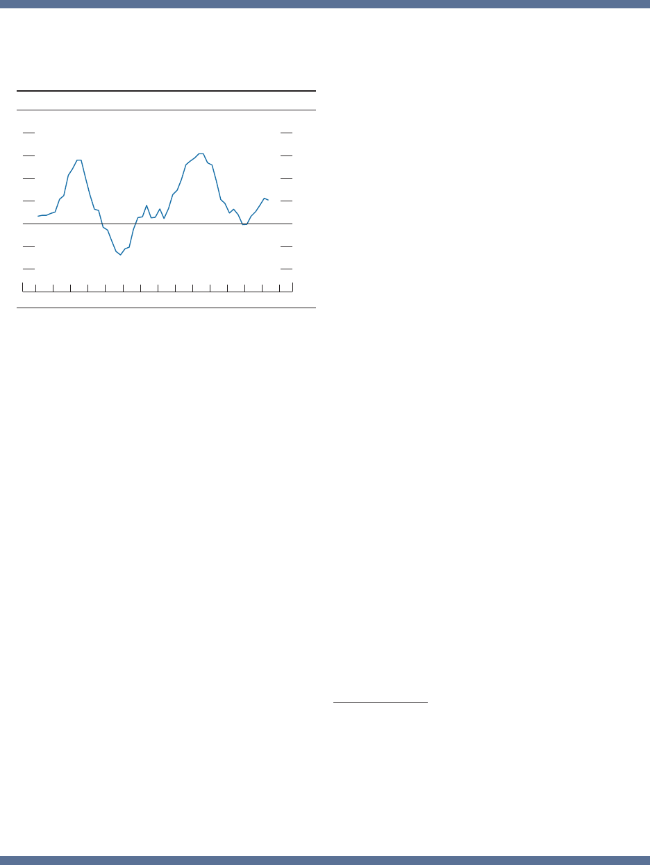
MONETARY POLICY REPORT: JULY 2018 27

a severe global recession.

The hypothetical “severely

adverse” scenario—the most stringent scenario

yet used in the Board’s stress tests, with the U.S.

unemployment rate rising almost 6percentage points to

10percent—projects $578billion in total losses for the

35 participating banks during the nine quarters tested.

Since 2009, these rms have added about $800billion

in common equity capital. The Board also evaluates the

capital planning processes of the participating banks,

including the rms’ planned capital actions, such as

dividend payments and share buybacks.

The Board did

not object to the capital plans of 34 rms.Although

the recent U.S. tax legislation is expected to increase

banks’ post-tax earnings, and hence their ability

to accrete capital, it did lead to one-time losses,

decreasing banks’ capital ratios at the end of 2017, the

jumping-off point of the stress tests. In part because

of these effects, evident in text gure36, two rms

were required to maintain their capital distributions

at the levels they paid in recent years. Separately, one

rm will be required to address the management and

analysis of its counterparty exposure under stress. The

Board objected to the capital plan of one bank because

of qualitative concerns.

Vulnerabilities associated with liquidity and

maturity transformation—that is, the nancing of

illiquid assets or long-maturity assets with short-

maturity debt—continue to be low, owing in part to

liquidity regulations for banks and money market

reform. Large banks have strong liquidity positions,

because their use of core deposits as a source of

funding and their holdings of high-quality liquid

assets remain near historical highs, while their use of

short-term wholesale funding as a share of liabilities

is near historical lows. Since the money market fund

reforms implemented in October2016, assets under

management at prime funds, institutions that proved

vulnerable to runs in the past, have remained far below

pre-reform levels. In addition, the growth in alternative

short-term investment vehicles, which may have some

corporate credit conditions are favorable overall,

with low interest expenses and defaults, the elevated

leverage in this sector could result in higher future

default rates. In addition, weak protection from loan

covenants could reduce early intervention by lenders

and lower recovery rates for investors on default.

Investors may also be exposed to signicant repricing

risks because bond yields and credit risk premiums are

both low.

Vulnerabilities from nancial-sector leverage

continue to be relatively low. Core nancial

intermediaries, including large banks, insurance

companies, and broker-dealers, appear well positioned

to weather economic stress. Regulatory capital ratios for

the global systemically important banks have remained

well above the fully phased-in enhanced regulatory

requirements and are close to historical highs. Capital

levels at insurance companies and broker-dealers

also remain relatively robust by historical standards.

However, some indicators of hedge fund leverage in

the equity market, such as the provision of total margin

credit to equity investors, have risen to historically

elevated levels, and in the past few quarters dealers

have reportedly eased, on net, price terms to their

hedge fund clients.

The results of supervisory stress tests released in June

by the Federal Reserve Board conrm that the nation’s

largest banks are strongly capitalized and would be

able to lend to households and businesses even during

Billions of dollars

2018201620142012201020082006

B. Total net issuance of risky debt

Quarterly

NOTE: Data are 4-quarter moving averages and extend through

2018:Q2.

Total

net issuance of risky debt is the sum of the net issuance

speculative-grade and unrated bonds and leveraged loans.

SOURCE

: Mergent Fixed Investment Securities Database, S&P

Leveraged

Commentary & Data.

2. See Board of Governors of the Federal Reserve System

(2018), “Federal Reserve Board Releases Results of Supervisory

Bank Stress Tests,” press release, June21, https://www.

federalreserve.gov/newsevents/pressreleases/

bcreg20180621a.htm.

3. See Board of Governors of the Federal Reserve System

(2018), “Federal Reserve Releases Results of Comprehensive

Capital Analysis and Review (CCAR),” press release, June29,

https://www.federalreserve.gov/newsevents/pressreleases/

bcreg20160629a.htm.

(continued on next page)

28 PART 1: RECENT ECONOMIC AND FINANCIAL DEVELOPMENTS

4. See Board of Governors of the Federal Reserve System

(2016), “Regulatory Capital Rules: The Federal Reserve Board’s

Framework for Implementing the U.S. Basel III Countercyclical

Capital Buffer,” nal policy statement (Docket No. R-1529),

Federal Register, vol. 81 (September16), pp. 63682–88.

similar vulnerabilities, continues to be limited, as

investors have shifted primarily from prime funds into

government funds.

Risks from abroad are moderate overall. Advanced

foreign economies (AFEs), many of which have

signicant nancial and real linkages to the United

States, continue to have notable or elevated valuations

in some asset markets and, in a few countries, high

levels of household debt relative to GDP. These

factors have contributed to some AFEs announcing

or implementing macroprudential actions, including

increases in countercyclical capital buffers, over the

past couple of years. More generally, AFE nancial

sectors continue their slow pace of deleveraging

that started after the global nancial and euro-area

sovereign debt crises. In addition, low corporate debt

spreads in the past few years have yet to translate

into any marked increase in leverage in most of these

countries’ nonnancial corporate sectors. Some major

emerging market economies continue to harbor

more pronounced vulnerabilities, reecting some

combination of the following: substantial corporate

leverage, scal concerns, or excessive reliance on

foreign funding. Globally, potential downside risks to

international nancial markets and nancial stability

include political uncertainty, an intensication of trade

tensions, and challenges posed by rising interest rates.

The countercyclical capital buffer (CCyB) is a

macroprudential tool the Federal Reserve Board can

use to increase the resilience of the nancial system

by raising capital requirements on the largest banks.

Activating the CCyB is appropriate when systemic

vulnerabilities are meaningfully above normal.

The

Board is closely monitoring the level and conguration

of systemic vulnerabilities described earlier.

Financial Stability (continued)

MONETARY POLICY REPORT: JULY 2018 29

also generally stable. Overall, the functioning

of Treasury and agency MBS markets has not

been materially aected by the implementation

of the Federal Reserve’s balance sheet

normalization program, including the

accompanying reduction in reinvestment of

principal payments from the Federal Reserve’s

securities holdings. Credit conditions in

municipal bond markets have remained stable

since the turn of the year. Over that period,

yield spreads on 20-year general obligation

municipal bonds over comparable-maturity

Treasury securities edged up a bit.

Money market rates have moved up in

line with increases in the FOMC’s target

range

Conditions in domestic short-term funding

markets have also remained generally stable

so far in 2018. Yields on a broad set of money

market instruments moved higher in response

to the FOMC’s policy actions in March and

June. Some money market rates rose during

the rst quarter more than what would

normally occur with monetary tightening.

For example, the spreads of certicates of

deposit and term London interbank oered

rates relative to overnight index swap (OIS)

rates increased notably, reportedly reecting

increased issuance of Treasury bills and

perhaps also the anticipated tax-induced

repatriation of foreign earnings by U.S.

corporations. The upward pressure on short-

term funding rates, beyond that driven by

expected monetary policy, eased in recent

months, leading to a narrowing of spreads

of some money market rates to OIS rates.

However, the spreads remain wider than at the

beginning of the year.

Bank credit continued to expand and

bank protability improved

Aggregate credit provided by commercial

banks continued to increase through the rst

quarter of 2018 at a pace similar to the one

seen in 2017. Its pace was slower than that of

nominal GDP, thus leaving the ratio of total

commercial bank credit to current-dollar

30 PART 1: RECENT ECONOMIC AND FINANCIAL DEVELOPMENTS

GDP slightly lower than in the previous year

(gure35). Available data for the second

quarter suggest that growth in banks’ core

loans continued to be moderate. Measures of

bank protability improved in the rst quarter

of 2018 after having experienced a temporary

decline in the last quarter of 2017. Weaker

fourth-quarter measures of bank protability

were partly driven by higher write-downs of

deferred tax assets in response to the U.S. tax

legislation (gure36).

International Developments

Political developments and signs of

moderating growth weighed on advanced

foreign economy asset prices

Since February, political developments

in Europe and moderation in economic

growth outside of the United States weighed

on some risky asset prices in advanced

foreign economies (AFEs). Interest rates on

sovereign bonds in several countries in the

European periphery rose notably relative to

core countries, and European bank shares

came under pressure, as investors focused

on the formation of the Italian government.

Nonetheless, peripheral bond spreads

remained well below their levels at the height

of the euro-area crisis, and the moves partly

retraced as a government was put in place.

Broad stock price indexes were little changed

on net (gure37). In contrast to the United

States, long-term sovereign yields and market-

implied paths of policy rates in the core euro

area as well as the United Kingdom declined

somewhat, and rates were little changed in

Japan (gure38).

Heightened investor focus on

vulnerabilities in emerging market

economies led asset prices to come under

pressure

Investor concerns about nancial

vulnerabilities in several emerging market

economies (EMEs) intensied this spring

against the backdrop of rising U.S. interest

rates. Broad measures of EME sovereign

United Kingdom

Euro area

100

110

120

130

140

Week ending January 7, 2015 = 100

2018201720162015

37. Equity indexes for selected foreign economies

Weekly

Emerging market economies

OTE

: The data are weekly averages of daily data and extend

through

July 11, 2018.

OURCE: For euro area, DJ Euro Stoxx Index; for United Kingdom,

FTSE

100

Stock Index; for emerging market economies, MSCI Emerging

Markets

Local Currency Index; all via Bloomberg.

Return on assets

Percent, annual rate

2.0

1.5

1.0

1.5

2.0

2018201620142012201020082006200420022000

36. Profitability of bank holding companies

Percent, annual rate

Return on equity

OTE

: The data are quarterly and are seasonally adjusted.

OURCE

: Federal Reserve Board, Form FR Y-9C, Consolidated

Financial

Statements for Bank Holding Companies.

Percent

2018201620142012201020082006200420022000

35. Ratio of total commercial bank credit to nominal gross

domestic product

Quarterly

SOURCE

: Federal Reserve Board, Statistical Release H.8, “Assets

and

Liabilities

of Commercial Banks in the United States”; Bureau of

Economic

Analysis via Haver Analytics.

MONETARY POLICY REPORT: JULY 2018 31

bond spreads over U.S. Treasury yields

widened notably, and benchmark EME equity

indexes declined, as investors scrutinized

macroeconomic policy approaches in several

countries. Turkey and Argentina, which faced

persistently high ination, expansionary scal

policies, and large current account decits,

were among the worst performers. Trade

policy developments between the United

States and its trading partners also weighed on

EME asset prices, especially on stock prices

in China and some emerging Asian countries.

EME mutual funds saw net outows in May

and June after generally solid inows earlier

in the year (gure39). While movements in

asset prices and capital ows were notable for

a number of economies, broad indicators of

nancial stress in EMEs remained low relative

to levels seen during other periods of stress in

recent years.

The dollar appreciated

After depreciating during 2017, the broad

exchange value of the U.S. dollar has

appreciated moderately in recent months

(gure40). Factors contributing to the

appreciation of the dollar likely include

moderating growth in some foreign economies

combined with continued output strength

and ongoing policy tightening in the United

States, downside risks stemming from political

developments in Europe and several EMEs,

and the recent developments in trade policy.

Several currencies appeared particularly

sensitive to trade policy developments,

including the Canadian dollar and the

Mexican peso, related to the North American

Free Trade Agreement negotiations, as well

as the Chinese renminbi, which fell notably

against the dollar in June.

The pace of economic activity moderated

in the AFEs

In the rst quarter, real GDP growth

decelerated in all major AFEs and turned

negative in Japan, down from robust rates of

activity in 2017 (gure41). Part of this slowing

is a result of temporary factors, though,

EMBI+ (left axis)

Billions of dollars

200

250

300

350

400

450

500

2018201720162015

39. Emerging market mutual fund flows and spreads

Basis points

Apr.

June

OTE

: The bond and equity fund flow data are quarterly sums of

weekly

data from January 1, 2015, to March 31, 2018, and monthly sums of

weekly

data from April 1, 2018, to June 30, 2018. The fund flows data exclude funds

located in China. The J.P. Morgan Emerging Markets Bond Index

Plus

(EMBI+) data are weekly averages of daily data and extend through July

2018.

OURCE

: For bond and equity fund flows, EPFR Global; for EMBI+,

J.P.

Morgan Emerging Markets Bond Index Plus via Bloomberg.

Bond fund flows (right axis)

Equity fund flows (right axis)

United Kingdom

Japan

Germany

1.0

1.5

2.0

2.5

3.0

Percent

2015 2016 2017 2018

38. Nominal 10-year government bond yields in

selected advanced economies

Weekly

United States

OTE: The data are weekly averages of daily benchmark yields and

extend

through July 11, 2018.

OURCE

:Bloomberg.

32 PART 1: RECENT ECONOMIC AND FINANCIAL DEVELOPMENTS

including unusually cold weather in Japan

and the United Kingdom, labor strikes in the

euro area, and disruptions in oil production in

Canada. In most AFEs, economic indicators

for the second quarter, including purchasing

manager surveys and exports, are generally

consistent with solid economic growth.

Despite tight labor markets,

ination pressures remain subdued in

most AFEs . . .

Sustained increases in oil prices provided

upward pressure on consumer price ination

across all AFEs in the rst half of the year

(gure42). However, core ination has

generally remained muted in most AFEs,

despite further improvement in labor market

conditions. In Canada, in contrast, core

ination picked up amid solid wage growth,

pushing the total ination rate above the

central bank target.

. . . prompting central banks to maintain

highly accommodative monetary policies

With underlying ination still subdued, the

Bank of Japan and the European Central

Bank (ECB) kept their policy rates at

historically low levels, although the ECB

indicated it would again reduce the pace of

its asset purchases starting in October. The

Bank of England and the Bank of Canada,

which both began raising interest rates last

year, signaled that further rate increases will

be gradual, given a moderation in the pace of

economic activity.

In emerging Asia, growth remained

solid . . .

Economic growth in China remained solid

in the rst quarter of 2018, as a rebound in

steel production and strong external demand

bolstered a recovery in industrial activity

and overall growth (gure43). Indicators

of investment and retail sales have slowed

in recent months, however, suggesting that

the authorities’ eort to rein in credit may

have softened domestic demand. Most other

Percent, annual rate

20182017201620152014

41. Real gross domestic product growth in selected

advanced foreign economies

OURCE:

For the United Kingdom, Office for National Statistics; for Japan,

Cabinet Office, Government of Japan; for the euro area, Eurostat; for

Canada,

Statistics Canada; all via Haver Analytics.

United Kingdom

Japan

Euro area

Canada

British pound

Mexican peso

Euro

100

110

120

130

140

150

Week ending January 7, 2015 = 100

2018201720162015

40. U.S. dollar exchange rate indexes

Weekly

Dollar appreciation

Broad dollar

OTE

: The data, which are in foreign currency units per dollar, are

weekly

averages of daily data and extend through July 11, 2018. As indicated by

the

arrow, increases in the data represent U.S. dollar appreciation, and

decreases

represent U.S. dollar depreciation.

OURCE: Federal Reserve Board, Statistical Release H.10,

“Foreign

Exchange Rates.”

MONETARY POLICY REPORT: JULY 2018 33

emerging Asian economies registered strong

growth in the rst quarter of 2018, partly

reecting solid external demand.

. . . while growth in some Latin American

economies was mixed

In Mexico, real GDP surged in the rst quarter

as economic activity rebounded from two

major earthquakes and a hurricane last year.

Following a brief recovery in the rst half of

2017, Brazil’s economy stalled in the fourth

quarter and grew tepidly in the rst quarter,

and a truckers’ strike paralyzed economic

activity in late May.

Percent, annual rate

20182017201620152014

43. Real gross domestic product growth in selected

emerging market economies

OTE

: The data for China are seasonally adjusted by Board staff. The data

for

Korea, Mexico, and Brazil are seasonally adjusted by their respective

government agencies.

SOURCE

: For China, China National Bureau of Statistics; for Korea, Bank

Korea; for Mexico, Instituto Nacional de Estadistica y Geografia; for

Brazil, Instituto Brasileiro de Geografia e Estatistica; all via Haver Analytics.

China

Korea

Mexico

Brazil

United Kingdom

Japan

Euro area

12-month percent change

2018201720162015

42. Consumer price inflation in selected advanced foreign

economies

Monthly

Canada

OTE

: The data for the euro area incorporate the flash estimate for

June

2018. The data for Canada, Japan, and the United Kingdom extend

through

May 2018.

OURCE

For the United Kingdom, Office for National Statistics; for Japan,

Ministry of International Affairs and Communications; for the euro

area,

Statistical Office of the European Communities; for Canada,

Statistics

Canada; all via Haver Analytics.

The Federal Open Market Committee

continued to gradually increase the

federal funds target range in the rst half

of the year . . .

Since December2015, the Federal Open

Market Committee (FOMC) has been

gradually increasing its target range for

the federal funds rate as the economy has

continued to make progress toward the

Committee’s congressionally mandated

objectives of maximum employment and

price stability. In the rst half of this year, the

Committee continued this gradual process of

scaling back monetary policy accommodation,

increasing its target range for the federal funds

rate ¼percentage point at its meetings in both

March and June. With these increases, the

federal funds rate is currently in the range of

1¾ to 2percent (gure44).

The Committee’s

decisions reected the continued strengthening

14. See Board of Governors of the Federal

Reserve System (2018), “Federal Reserve Issues

FOMC Statement,” press release, March21, https://

www.federalreserve.gov/newsevents/pressreleases/

monetary20180321a.htm; and Board of Governors of

the Federal Reserve System (2018), “Federal Reserve

Issues FOMC Statement,” press release, June13, https://

www.federalreserve.gov/newsevents/pressreleases/

monetary20180613a.htm.

of the labor market and the accumulating

evidence that, after many years of running

below the Committee’s 2percent longer-

run objective, ination had moved close to

2percent.

. . . but monetary policy continues to

support economic growth

Even after the gradual increases in the federal

funds rate over the rst half of the year, the

Committee judges that the stance of monetary

policy remains accommodative, thereby

supporting strong labor market conditions

and a sustained return to 2percent ination.

In particular, the federal funds rate remains

somewhat below most FOMC participants’

estimates of its longer-run value.

The Committee expects that a gradual

approach to increasing the target range for

the federal funds rate will be consistent with

a sustained expansion of economic activity,

strong labor market conditions, and ination

near the Committee’s symmetric 2percent

objective over the medium term. Consistent

with this outlook, in the most recent

Summary of Economic Projections (SEP),

which was compiled at the time of the June

FOMC meeting, the median of participants’

Part 2

monetary PoLicy

Target federal funds rate

2-year Treasury rate

Percent

2008 2009 2010 2011 2012 2013 2014 2015 2016 2017 2018

44. Selected interest rates

Daily

10-year Treasury rate

OTE

: The 2-year and 10-year Treasury rates are the constant-maturity yields based on the most actively traded securities.

SOURCE

: Department of the Treasury; Federal Reserve Board.

36 PART 2: MONETARY POLICY

assessments for the appropriate level of the

target range for the federal funds rate at

year-end rises gradually over the period from

2018 to 2020 and stands somewhat above the

median projection for its longer-run level by

the end of 2019 and through 2020.

Future changes in the federal funds rate

will depend on the economic outlook as

informed by incoming data

The FOMC has continued to emphasize

that, in determining the timing and size of

future adjustments to the target range for

the federal funds rate, it will assess realized

and expected economic conditions relative

to its maximum-employment objective and

its symmetric 2percent ination objective.

This assessment will take into account a wide

range of information, including measures

of labor market conditions, indicators of

ination pressures and ination expectations,

and readings on nancial and international

developments.

In evaluating the stance of monetary policy,

policymakers routinely consult prescriptions

from a variety of policy rules, which can serve

15. See the June SEP, which appeared as an addendum

to the minutes of the June12–13, 2018, meeting of the

FOMC and is presented in Part 3 of thisreport.

as useful benchmarks. However, the use and

interpretation of such prescriptions require,

among other considerations, careful judgments

about the choice and measurement of the

inputs to these rules such as estimates of the

neutral interest rate, which are highly uncertain

(see the box “Complexities of Monetary

PolicyRules”).

The FOMC has continued to implement

its program to gradually reduce the

Federal Reserve’s balance sheet

The Committee has continued to implement

the balance sheet normalization program

described in the June2017 Addendum to the

Policy Normalization Principles and Plans.

This program is gradually and predictably

reducing the Federal Reserve’s securities

holdings by decreasing the reinvestment of the

principal payments it receives from securities

held in the System Open Market Account.

Since the initiation of the balance sheet

normalization program in October of last year,

such payments have been reinvested to the

extent that they exceeded gradually rising caps

(gure45).

16. The addendum, adopted on June13, 2017, is

available at https://www.federalreserve.gov/monetarypolicy/

files/FOMC_PolicyNormalization.20170613.pdf.

45. Principal payments on SOMA securities

N: Reinvestment and redemption amounts of agency mortgage-backed securities are projections starting in June 2018. The data

extend through December 2019.

S: Federal Reserve Bank of New York; Federal Reserve Board sta calculations.

Agency debt and mortgage-backed securities Treasury securities

Billions of dollarsMonthly

201920182017

Monthly cap

Redemptions

Reinvestments

201920182017

Monthly cap

Redemptions

Reinvestments

MONETARY POLICY REPORT: JULY 2018 37

(continued on next page)

reect the three key principles of good monetary policy

noted earlier. Each rule takes into account estimates

of how far the economy is from achieving the Federal

Reserve’s dual-mandate goals of maximum employment

and price stability.

Four of the ve rules include the difference

between the rate of unemployment that is sustainable

in the longer run and the current unemployment

rate (the unemployment rate gap); the rst-difference

rule includes the change in the unemployment gap

rather than its level.

In addition, four of the ve rules

include the difference between recent ination and the

FOMC’s longer-run objective (2percent as measured

by the annual change in the price index for personal

consumption expenditures, or PCE), while the price-

level rule includes the gap between the level of prices

today and the level of prices that would be observed

if ination had been constant at 2percent from a

specied starting year (PLgap

The price-level rule

thereby takes account of the deviation of ination from

Overview

Monetary policy rules are mathematical formulas

that relate a policy interest rate, such as the federal

funds rate, to a small number of other economic

variables—typically including the deviation of ination

from its target value along with an estimate of resource

slack in the economy. Policy rules can provide helpful

guidance for policymakers. Indeed, since 2004,

prescriptions from policy rules have been included

in written materials that are routinely sent to the

Federal Open Market Committee (FOMC). However,

interpretation of the prescriptions of policy rules

requires careful judgment about the measurement of

the inputs to the rules and the implications of the many

considerations that the rules do not take into account.

Policy rules can incorporate key principles of good

monetary policy.

One key principle is that monetary

policy should respond in a predictable way to changes

in economic conditions. A second key principle is

that monetary policy should be accommodative when

ination is below the desired level and employment

is below its maximum sustainable level; conversely,

monetary policy should be restrictive when the

opposite holds. A third key principle is that, to stabilize

ination, the policy rate should be adjusted by more

than one-for-one in response to persistent increases or

decreases in ination.

Economists have analyzed many monetary policy

rules, including the well-known Taylor (1993) rule.

Other rules include the “balanced approach” rule, the

“adjusted Taylor (1993)” rule, the “price level” rule, and

the “rst difference” rule (gure A).

These policy rules

Complexities of Monetary Policy Rules

1. For discussion regarding principles for the conduct of

monetary policy and monetary policy rules, see Board of

Governors of the Federal Reserve System (2018), “Monetary

Policy Principles and Practice,” Board of Governors, https://

www.federalreserve.gov/monetarypolicy/monetary-policy-

principles-and-practice.htm.

2. The Taylor (1993) rule was suggested in John B. Taylor

(1993), “Discretion versus Policy Rules in Practice,” Carnegie-

Rochester Conference Series on Public Policy, vol.39

(December), pp. 195–214. The balanced-approach rule was

analyzed in John B. Taylor (1999), “A Historical Analysis of

Monetary Policy Rules,” in John B. Taylor, ed., Monetary Policy

Rules (Chicago: University of Chicago Press), pp.319–41. The

adjusted Taylor (1993) rule was studied in David Reifschneider

and John C. Williams (2000), “Three Lessons for Monetary

Policy in a Low-Ination Era,” Journal of Money, Credit and

Banking, vol. 32 (November), pp. 936–66. A price-level rule

was discussed in Robert E. Hall (1984), “Monetary Strategy

with an Elastic Price Standard,” in Price Stability and Public

Policy, proceedings of a symposium sponsored by the Federal

Reserve Bank of Kansas City, held in Jackson Hole, Wyo.,

August2–3 (Kansas City: Federal Reserve Bank of Kansas

City), pp. 137–59, https://www.kansascityfed.org/publicat/

sympos/1984/s84.pdf. Finally, the rst-difference rule was

introduced by Athanasios Orphanides (2003), “Historical

Monetary Policy Analysis and the Taylor Rule,” Journal

of Monetary Economics, vol. 50 (July), pp. 983–1022. A

comprehensive review of policy rules is in John B. Taylor

and John C. Williams (2011), “Simple and Robust Rules for

Monetary Policy,” in Benjamin M. Friedman and Michael

Woodford, eds., Handbook of Monetary Economics, vol.3B

(Amsterdam: North-Holland), pp. 829–59. The same volume

of the Handbook of Monetary Economics also discusses

approaches other than policy rules for deriving policy rate

prescriptions.

3. The Taylor (1993) rule represented slack in resource

utilization using an output gap (the difference between the

current level of real gross domestic product (GDP) and what

GDP would be if the economy was operating at maximum

employment). The rules in gure A represent slack in resource

utilization using the unemployment gap instead, because that

gap better captures the FOMC’s statutory goal to promote

maximum employment. Movements in these alternative

measures of resource utilization are highly correlated. For

more information, see the note below gure A.

4. Calculating the prescriptions of the price-level rule

requires selecting a starting year for the price level from which

to cumulate the 2percent annual ination. Figure B uses 1998

as the starting year. Around that time, the underlying trend

of ination and longer-term ination expectations stabilized

at a level consistent with PCE price ination being close to

2percent.

38 PART 2: MONETARY POLICY

Monetary Policy Rules (continued)

also recognizes that the federal funds rate cannot be

reduced materially below zero. If ination runs below

the 2percent objective during periods when the rule

prescribes setting the federal funds rate well below

zero, the price-level rule will, over time, provide

accommodation to make up for the past ination

shortfall.

The U.S. economy is complex, and the monetary

policy rules shown in gure A do not capture many

elements that are relevant to the conduct of monetary

policy. Moreover, as shown in gure B, different

monetary policy rules often offer quite different

prescriptions for the federal funds rate.

In practice,

there is no unique criterion for favoring one rule over

another. In recent years, almost all of the policy rules

the long-run objective in earlier periods as well as

the current period. Thus, if ination had been running

persistently above 2percent, the price-level rule would

prescribe a higher level for the federal funds rate than

rules that use the current ination gap. Likewise,

if ination had been running persistently below

2percent, the price-level rule would prescribe setting

the policy rate lower than rules that use the current

ination gap.

The adjusted Taylor (1993) rule recognizes that

the federal funds rate cannot be reduced materially

below zero, and that following the prescriptions

of the standard Taylor (1993) rule after a recession

during which interest rates have fallen to their lower

bound may, for a time, not provide enough policy

accommodation. To make up for the cumulative

shortfall in accommodation (Z

), the adjusted rule

prescribes only a gradual return of the policy rate to

the (positive) levels prescribed by the standard Taylor

(1993) rule after the economy begins to recover.

The particular price-level rule specied in gure A

Taylor (1993) rule

= + +0.5

(

−

)

− )

= + +0.5

(

−

)

+2(

− )

Taylor (1993) rule, adjusted

= {

− , 0}

= { + +

(

−

)

+0.5

( ), 0}

−1

+0.5

(

−

)

(

−

)

−(

−4

−

−4

)

A. Monetary policy rules

Balanced-approach rule

Price-level rule

First-dierence rule

N: R

T93

, R

T93adj

, R

, and R

represent the values of the nominal federal funds rate prescribed by the Taylor (1993),

balanced-approach, adjusted Taylor (1993), price-level, and rst-dierence rules, respectively.

denotes the actual nominal federal funds rate for quarter t, π

is four-quarter price ination for quarter t, u

is the

unemployment rate in quarter

t, and r

is the level of the neutral real federal funds rate in the longer run that, on average, is

expected to be consistent with sustaining maximum employment and ination at the FOMC’s 2 percent longer-run objective,

. In addition, u

is the rate of unemployment in the longer run. Z

is the cumulative sum of past deviations of the federal

funds rate from the prescriptions of the Taylor (1993) rule when that rule prescribes setting the federal funds rate below zero

PLgap

is the percent deviation of the actual level of prices from a price level that rises 2 percent per year from its level in a

specied starting period.

The Taylor (1993) rule and other policy rules are generally written in terms of the deviation of real output from its full

capacity level. In these equations, the output gap has been replaced with the gap between the rate of unemployment in the

longer run and its actual level (using a relationship known as Okun’s law) in order to represent the rules in terms of the

FOMC’s statutory goals. Historically, movements in the output and unemployment gaps have been highly correlated. Box

note 2 provides references for the policy rules.

5. These prescriptions are calculated using (1) published

data for ination and the unemployment rate and (2)

survey-based estimates of the longer-run value of the

neutral real interest rate and the longer-run value of the

unemploymentrate.

(continued)

MONETARY POLICY REPORT: JULY 2018 39

(continued on next page)

growth, changing demographics, and other shifts in the

structure of the economy. As a result, estimates of the

neutral real interest rate in the longer run made today

may differ substantially from estimates made later.

Academic studies have estimated the longer-

run value of the neutral real interest rate using

statistical techniques to capture the variations among

ination, interest rates, real gross domestic product,

unemployment, and other data series. The range of

estimates is wide but suggests that the neutral real rate

has declined since the turn of the century (gure C).

There is substantial statistical uncertainty surrounding

each estimate of the longer-run value of the neutral

real rate, as evidenced by the width of the 95percent

shown have called for rising values of the federal funds

rate, but the pace of tightening that the rules prescribe

has varied widely.

Uncertainty about the neutral interest rate

in the longer run

The Taylor (1993), balanced-approach, adjusted

Taylor (1993), and price-level rules provide

prescriptions for the level of the federal funds rate;

all require an estimate of the neutral real interest rate

in the longer run (r

)—that is, the level of the real

federal funds rate that is expected to be consistent, in

the longer run, with maximum employment and stable

ination.

The neutral real interest rate in the longer

run is determined by structural features of the economy

and is not observable. In addition, its value may vary

over time because of uctuations in trend productivity

First-difference rule

Price-level ruleTarget federal funds rate

Balanced-approach rule

Taylor (1993) rule, adjusted

Percent

2018201620142012201020082006200420022000

B. Historical federal funds rate prescriptions from simple policy rules

Quarterly

Taylor (1993) rule

OTE: The rules use historical values of inflation, the federal funds rate, and the unemployment rate. Inflation is measured as the 4-quarter percent change

the

price index for personal consumption expenditures (PCE) excluding food and energy. Quarterly projections of long-run values for the federal funds rate

and

the

unemployment rate are derived through interpolations of biannual projections from Blue Chip Economic Indicators. The long-run value for inflation is

taken

2 percent. The target value of the price level is the average level of the price index for PCE excluding food and energy in 1998 extrapolated at 2 percent

per

year.

OURCE

: Federal Reserve Bank of Philadelphia; Wolters Kluwer, Blue Chip Economic Indicators; Federal Reserve Board staff estimates.

6. The rst-difference rule shown in gure A does not

require an estimate of the neutral real interest rate in the

longer run. However, this rule has its own shortcomings. For

example, research suggests that this sort of rule will result in

greater volatility in employment and ination relative to what

would be obtained under the Taylor (1993) and balanced-

approach rules unless the estimates of the neutral real federal

funds rate in the longer run and the rate of unemployment in

the longer run that are included in those rules are sufciently

far from their true values.

7. The range of estimates is computed using published

values or values computed using the methodology from the

following studies: Marco Del Negro, Domenico Giannone,

Marc P. Giannoni, and Andrea Tambalotti (2017), “Safety,

Liquidity, and the Natural Rate of Interest,” Brookings

Papers on Economic Activity, Spring, pp. 235–94, https://

www.brookings.edu/wp-content/uploads/2017/08/

delnegrotextsp17bpea.pdf; Kathryn Holston, Thomas Laubach,

and John C. Williams (2017), “Measuring the Natural

Rate of Interest: International Trends and Determinants,”

Journal of International Economics, supp. 1, vol. 108

(May), pp.S59–75; Benjamin K. Johannsen and Elmar

Mertens (2016), “The Expected Real Interest Rate in the

Long Run: Time Series Evidence with the Effective Lower

Bound,” FEDS Notes (Washington: Board of Governors

40 PART 2: MONETARY POLICY

uncertainty bands for the estimated values in the rst

quarter of 2018 (gure D).

The longer-run normal level of the federal funds

rate under appropriate monetary policy—equal to

the sum of the neutral real interest rate in the longer

run and the FOMC’s 2percent ination objective—is

one benchmark for evaluating the current stance

of monetary policy. Uncertainty about the longer-

run value of the neutral real interest rate leads to

uncertainty about how far the current federal funds

rate is from its longer-run normal level. For the Taylor

(1993), balanced-approach, adjusted Taylor (1993), and

price-level rules, different estimates of the neutral real

interest rate in the longer run translate one-for-one to

differences in the prescribed setting of the federal funds

rate. As a result, the substantial statistical uncertainty

accompanying estimates of the neutral rate in the

longer run implies substantial uncertainty surrounding

the prescriptions of each policy rule. Following the

prescriptions of a policy rule with an incorrect value of

the neutral rate could lead to poor economic outcomes.

If the longer-run value of the neutral real interest rate

is currently at the low end of the range of estimates,

of the Federal Reserve System, February9), https://www.

federalreserve.gov/econresdata/notes/feds-notes/2016/

the-expected-real-interest-rate-in-the-long-run-time-series-

evidence-with-the-effective-lower-bound-20160209.html;

Michael T. Kiley (2015), “What Can the Data Tell Us about

the Equilibrium Real Interest Rate?” Finance and Economics

Discussion Series 2015-77 (Washington: Board of Governors

of the Federal Reserve System, September), http://dx.doi.

org/10.17016/FEDS.2015.077; Thomas Laubach and John

C. Williams (2015), “Measuring the Natural Rate of Interest

Redux,” Hutchins Center Working Paper 15 (Washington:

Brookings Institution, November), https://www.brookings.

edu/wp-content/uploads/2016/07/WP15-Laubach-Williams-

natural-interest-rate-redux.pdf; Kurt F. Lewis and Francisco

Vazquez-Grande (2017), “Measuring the Natural Rate of

Interest: Alternative Specications,” Finance and Economics

Discussion Series 2017-059 (Washington: Board of

Percent

2018201520122009200620032000

C. Range of selected estimates for the neutral real federal

funds rate in the longer run

Quarterly

NOTE: The shaded bars indicate periods of business recession as defined

the National Bureau of Economic Research.

SOURCE: Federal Reserve Board staff calculations, along with

references

listed in box note 7.

Range of selected estimates

Monetary Policy Rules (continued)

then monetary policy is more likely to be constrained

by the lower bound on nominal interest rates in the

future. Historically, the FOMC has cut the federal

funds rate by 5percentage points, on average, during

downturns in the economy. Cutting the federal funds

rate by this much in response to a future economic

downturn may not be feasible if the neutral federal

funds rate is as low as most of the estimates suggest.

Governors of the Federal Reserve System, June), https://

doi.org/10.17016/FEDS.2017.059; Thomas A. Lubik and

Christian Matthes (2015), “Calculating the Natural Rate of

Interest: A Comparison of Two Alternative Approaches,”

Economic Brief 15-10 (Richmond, Va.: Federal Reserve Bank

of Richmond, October), https://www.richmondfed.org/-/media/

richmondfedorg/publications/research/economic_brief/2015/

pdf/eb_15-10.pdf.

(continued)

MONETARY POLICY REPORT: JULY 2018 41

D. Point estimates and uncertainty bands for neutral real rate in the longer run as of 2018:Q1

Study Point estimate

95percent uncertainty band

Del Negro and others (2017)

1.3 (.7, 2.1)

Holston and others (2017) .6

(-2.5, 3.7)

Johannsen and Mertens (2016) .7 (-1.3, 2.5)

Kiley (2015) .4 (-.6, 1.6)

Laubach and Williams (2015) .1 (-5.4, 5.6)

Lewis and Vazquez-Grande (2017) 1.8 (.5, 3.1)

Lubik and Matthes (2015) 1.0 (-2.3, 4.5)

S: Federal Reserve Board sta calculations, along with references listed in box note7.

As a result, it may not be feasible to provide the levels

of accommodation prescribed by many policy rules,

potentially leading to elevated unemployment and

ination averaging below the Committee’s 2percent

objective.

Rules that try to offset the cumulative

shortfall of accommodation posed by the lower bound

on nominal interest rates, such as the adjusted Taylor

(1993) rule, or make up the cumulative shortfall in

the level of prices, such as the price-level rule, are

intended to mitigate the effects of the lower bound

on the economy by providing more accommodation

than prescribed by rules that do not have these

makeupfeatures.

In the years following the nancial crisis, with the

federal funds rate close to zero, the FOMC recognized

that it would have limited scope to respond to an

unexpected weakening in the economy by lowering

short-term interest rates. This risk has, in recent years,

provided a sound rationale for following a more

gradual path of rate increases than that prescribed by

some policy rules. In these circumstances, increasing

the policy rate quickly in order to have room to

cut rates during an economic downturn could be

counterproductive because it might make a downturn

more likely to happen.

8. For further discussion of these issues, see Michael T.

Kiley and John M. Roberts (2017), “Monetary Policy in a Low

Interest Rate World,” Brookings Papers on Economic Activity,

Spring, pp. 317–72, https://www.brookings.edu/wp-content/

uploads/2017/08/kileytextsp17bpea.pdf.

9. Economists have found that a “makeup” policy can

be the best response in theory when the policy interest

rate is constrained at zero. See Ben S. Bernanke (2017),

“Monetary Policy in a New Era,” paper presented at

“Rethinking Macroeconomic Policy,” a conference held at the

Peterson Institute for International Economics, Washington,

October12–13, https://piie.com/system/les/documents/

bernanke20171012paper.pdf; and Michael Woodford (1999),

“Commentary: How Should Monetary Policy Be Conducted

in an Era of Price Stability?” in New Challenges for Monetary

Policy, proceedings of a symposium sponsored by the Federal

Reserve Bank of Kansas City (Kansas City, Mo.: Federal

Reserve Bank of Kansas City) pp. 277–316, https://www.

kansascityfed.org/publications/research/escp/symposiums/

escp-1999.

42 PART 2: MONETARY POLICY

In the rst quarter, the Open Market Desk

at the Federal Reserve Bank of New York,

as directed by the Committee, reinvested

principal payments from the Federal Reserve’s

holdings of Treasury securities maturing

during each calendar month in excess of

$12billion. The Desk also reinvested in agency

mortgage-backed securities (MBS) the amount

of principal payments from the Federal

Reserve’s holdings of agency debt and agency

MBS received during each calendar month in

excess of $8billion. Over the second quarter,

payments of principal from maturing Treasury

securities and from the Federal Reserve’s

holdings of agency debt and agency MBS were

reinvested to the extent that they exceeded

$18billion and $12billion, respectively. At

its meeting in June, the FOMC increased the

cap for Treasury securities to $24billion and

the cap for agency debt and agency MBS

to $16billion, both eective in July. The

Committee has indicated that the caps for

Treasury securities and for agency securities

will increase to $30billion and $20billion per

month, respectively, in October. These terminal

caps will remain in place until the Committee

judges that the Federal Reserve is holding no

more securities than necessary to implement

monetary policy eciently and eectively.

The implementation of the program has

proceeded smoothly without causing disruptive

price movements in Treasury and MBS

markets. As the caps have increased gradually

and predictably, the Federal Reserve’s total

assets have started to decrease, from about

$4.4trillion last October to about $4.3trillion

at present, with holdings of Treasury securities

at approximately $2.4trillion and holdings

of agency and agency MBS at approximately

$1.7trillion (gure46).

The Federal Reserve’s implementation of

monetary policy has continued smoothly

To implement the FOMC’s decisions to raise

the target range for the federal funds rate in

March and June of 2018, the Federal Reserve

increased the rate of interest on excess reserves

(IOER) along with the interest rate oered

on overnight reverse repurchase agreements

(ON RRPs). Specically, the Federal Reserve

increased the IOER rate to 1¾percent and

the ON RRP oering rate to 1½percent in

March. In June, the Federal Reserve increased

the IOER rate to 1.95percent—5 basis points

below the top of the target range—and the

ON RRP oering rate to 1¾percent. In

addition, the Board of Governors approved

Trillions of dollars

2008 2009 2010 2011 2012 2013 2014 2015 2016 2017 2018

46. Federal Reserve assets and liabilities

Weekly

Assets

Liabilities and capital

Other assets

Credit and liquidity

facilities

Agency debt and mortgage-backed securities holdings

Treasury securities held outright

Federal Reserve notes in circulation

Deposits of depository institutions

Capital and other liabilities

5.0

4.5

4.0

3.5

3.0

2.5

2.0

1.5

1.0

1.5

2.0

2.5

3.0

3.5

4.0

4.5

5.0

OTE: “Credit and liquidity facilities” consists of primary, secondary, and seasonal credit; term auction credit; central bank liquidity swaps; support

for

Maiden Lane, Bear Stearns, and AIG; and other credit facilities, including the Primary Dealer Credit Facility, the Asset-Backed Commercial Paper

Money

Market Mutual Fund Liquidity Facility, the Commercial Paper Funding Facility, and the Term Asset-Backed Securities Loan Facility. “Other

assets”

includes unamortized premiums and discounts on securities held outright. “Capital and other liabilities” includes reverse repurchase agreements, the

U.S.

Treasury General Account, and the U.S. Treasury Supplementary Financing Account. The data extend through July 4, 2018.

SOURCE: Federal Reserve Board, Statistical Release H.4.1, “Factors Affecting Reserve Balances.”

MONETARY POLICY REPORT: JULY 2018 43

a ¼percentage point increase in the discount

rate (the primary credit rate) in both March

and June. Yields on a broad set of money

market instruments moved higher, roughly in

line with the federal funds rate, in response

to the FOMC’s policy decisions in March

and June. Usage of the ON RRP facility

has declined, on net, since the turn of the

year, reecting relatively attractive yields on

alternative investments.

The eective federal funds rate moved up

toward the IOER rate in the months before

the June FOMC meeting and, therefore,

was trading near the top of the target range.

At its June meeting, the Committee made a

small technical adjustment in its approach

to implementing monetary policy by setting

the IOER rate modestly below the top of the

target range for the federal funds rate. This

adjustment resulted in the eective federal

funds rate running closer to the middle of the

target range since mid-June. In an environment

of large reserve balances, the IOER rate has

been an essential policy tool for keeping the

federal funds rate within the target range set by

the FOMC (see the box “Interest on Reserves

and Its Importance for Monetary Policy”).

44 PART 2: MONETARY POLICY

(continued)

As the economic expansion continued and

unemployment declined—and with labor market

conditions projected to continue improving—the

FOMC decided that it would scale back policy

support by increasing the level of short-term interest

rates and by reducing the Federal Reserve’s securities

holdings. To that end, the Committee began gradually

raising its target range for the federal funds rate in

December2015. Later, in October2017, it began

gradually reducing holdings of Treasury and agency

securities; this gradual reduction results in a decline in

the supply of reserve balances. The FOMC judged that

removing monetary policy stimulus through this mix of

rst raising the federal funds rate and then beginning

to shrink the balance sheet would best contribute to

achieving and maintaining maximum employment and

price stability without causing dislocations in nancial

markets or institutions that could put the economic

expansion at risk.

Interest on reserves—the payment of interest on

balances held by banks in their accounts at the Federal

Reserve—has been an essential policy tool that has

permitted the FOMC to achieve a gradual increase in

the federal funds rate in combination with a gradual

reduction in the Fed’s securities holdings and in the

supply of reserve balances.

Interest on reserves is a

monetary policy tool used by all of the world’s major

central banks.

Interest on reserves is the principal tool the FOMC

uses to anchor the federal funds rate in the target range.

The federal funds rate, in turn, establishes an important

benchmark for the borrowing and lending decisions

in the banking sector (gure A). When the Federal

Reserve increases the target range for the federal funds

rate and the interest rate it pays on reserve balances,

banks bid up the rates in short-term funding markets

to levels consistent with those increases; rates in other

short-term funding markets—such as commercial

paper rates, Treasury bill rates, and rates on repurchase

The nancial crisis that began in 2007 triggered the

deepest recession in the United States since the Great

Depression. In response, the Federal Open Market

Committee (FOMC) cut its target for the federal funds

rate to nearly zero by late 2008. Other short-term

interest rates declined roughly in line with the federal

funds rate. Additional monetary stimulus was necessary

to address the signicant economic downturn and

the associated downward pressure on ination. The

FOMC undertook other monetary policy actions to

put downward pressure on longer-term interest rates,

including large-scale purchases of longer-term Treasury

securities and agency-guaranteed mortgage-backed

securities.

These policy actions made nancial conditions more

accommodative and helped spur an economic recovery

that has become a long-lasting economic expansion.

The unemployment rate has declined from 10percent

to less than 4percent over the course of the recovery

and expansion, and ination has been low and fairly

stable. The FOMC’s actions were critical to fostering

progress toward maximum employment and stable

prices—the statutory goals for the conduct of monetary

policy established by the Congress.

The Federal Reserve’s large-scale asset purchases

had the side effect of generating a sizable increase in

the supply of reserve balances, which are the balances

that banks maintain in their accounts at the Federal

Reserve.

From the onset of the nancial crisis in

August2007 until October2014, when the FOMC

ended the last of its asset purchase programs, the

supply of reserve balances rose from about $15billion

to about $2½trillion.

Reserve balances rose well

above the level necessary to meet reserve requirements,

thus swelling the quantity of excess reserves held by the

banking system.

Interest on Reserves and Its Importance for Monetary Policy

1. All depository institutions (commercial banks, savings

banks, thrift institutions, credit unions, and most U.S. branches

and agencies of foreign banks) that maintain reserve balances

are eligible to earn interest on those balances. We refer to

these institutions as “banks.”

2. For a detailed discussion of how the changes in Federal

Reserve securities holdings affect the Federal Reserve’s

balance sheet and sectors of the U.S. economy, see Jane

Ihrig, Lawrence Mize, and Gretchen C. Weinbach (2017),

“How Does the Fed Adjust Its Securities Holdings and Who Is

Affected?” Finance and Economics Discussion Series 2017-

099 (Washington: Board of Governors of the Federal Reserve

System, September), https://www.federalreserve.gov/econres/

feds/les/2017099pap.pdf.

3. The Financial Services Regulatory Relief Act of 2006

authorized the Federal Reserve Banks to pay interest on

balances held by or on behalf of depository institutions at

Federal Reserve Banks, subject to regulations of the Board of

Governors, effective October1, 2011. The effective date of this

authority was changed to October1, 2008, by the Emergency

Economic Stabilization Act of 2008. The Congress authorized

the payment of interest on reserves to help minimize the

incentives for costly reserve avoidance schemes and to provide

the Federal Reserve with a policy tool that could be useful for

monetary policy implementation more broadly.

MONETARY POLICY REPORT: JULY 2018 45

is higher than the interest it pays on reserve balances.

Each year, the Federal Reserve remits its earnings—

that is, its income net of expenses—to the Treasury

Department; in 2017, remittances totaled more than

$80billion.

Had the Federal Reserve not been able to pay

interest on reserve balances at the same time that

excess reserves in the banking system were large, it

would not have been able to gradually raise the federal

funds rate and other short-term interest rates while

reserve balances were abundant; the FOMC would

have had to take a different approach to scaling back

monetary policy accommodation. This approach likely

would have involved a rapid and sizable reduction

in the Federal Reserve’s securities holdings in order

to put sufcient upward pressure on interest rates.

agreements—all tend to move higher as well (gure B).

This increase in the general level of short-term rates,

together with the expected future path of short-term

rates, then inuences the level of other nancial asset

prices and overall nancial conditions in the economy.

Thus, changing the interest rate on reserves has proven

to be an effective tool for transmitting changes in the

FOMC’s target range for the federal funds rate to other

interest rates in the economy.

The rate of interest the Federal Reserve pays on

banks’ reserve balances is far lower than the rate that

banks can earn on alternative safe assets, including

most U.S. government or agency securities, municipal

securities, and loans to businesses and consumers.

Indeed, the bank prime rate—the base rate that banks

use for loans to many of their customers—is currently

around 300 basis points above the level of interest on

reserves. Banks continue to nd lending attractive,

and bank lending has been expanding at a solid pace

since 2012. Households have begun to see interest

rates on retail deposits rising as well. Moreover, the

conguration of interest rates implies that the return

the Federal Reserve earns on its holdings of securities

Eurodollar

Treasury GCF repo

Federal funds

100

125

150

175

200

225

250

Basis points

201820172016

A. Overnight money market rates

Daily

Interest on reserves

NOTE: The upper bound of the target range is the interest on reserves

rate

until

June 13, 2018, after which it is 5 basis points higher. The federal

funds

and Eurodollar rates closely track one another over the period shown. GCF is

General Collateral Finance.

SOURCE: For Treasury GCF repo, DTCC Solutions LLC, an affiliate of

The

Depository

Trust & Clearing Corporation; for federal funds, Federal Reserv

Bank

of New York; for Eurodollar, Bloomberg; for interest on reserves

and

target range, Federal Reserve Board.

Target range

3-month Treasury bill

3-month AA financial

commercial paper

100

125

150

175

200

225

250

Basis points

201820172016

B. Term money market rates

Daily

Interest on reserves

NOTE: The upper bound of the target range is the interest on reserves

rate

until June 13, 2018, after which it is 5 basis points higher.

SOURCE: For U.S. Treasury bill, Department of the Treasury; for

financial

commercial paper, interest on reserves, and target range,

Federal

Reserve Board.

Target range

(continued on next page)

4. The Congress’s authorization allows the Federal

Reserve to pay interest on deposits maintained by depository

institutions at a rate not to exceed the “general level of

short-term interest rates.” The Federal Reserve Board’s

RegulationD denes short-term interest rates for the purposes

of this authority as “rates on obligations with maturities of

no more than one year, such as the primary credit rate and

rates on term federal funds, term repurchase agreements,

commercial paper, term Eurodollar deposits, and other similar

instruments.” The rate of interest on reserves has been well

within a range of short-term interest rates as dened in Board

regulations. For current rates on a number of short-term money

market instruments, see Board of Governors of the Federal

Reserve System, Statistical Release H.15, “Selected Interest

Rates,” www.federalreserve.gov/releases/h15/current.

46 PART 2: MONETARY POLICY

yet known, that level is likely to be much lower than it

is today, though appreciably higher than it was before

the crisis.

In addition, the amount of U.S. currency—

Federal Reserve notes—that people in the United States

and elsewhere want to hold has increased substantially

since the crisis. If banks want to hold more reserve

balances and the public wants to hold more U.S.

currency than before the crisis, the Federal Reserve will

need to supply the reserves and currency, so the Federal

Reserve’s securities holdings also will have to be larger

than before the nancial crisis.

Interest on reserves will remain an important policy

tool for keeping the federal funds rate within the target

range set by the FOMC and thus managing the level of

short-term interest rates, even as the ongoing reduction

in the Federal Reserve’s securities holdings generates a

gradual decline in the amount of reserve balances on

which the Federal Reserve pays interest. In June2018,

the Federal Reserve made a small technical adjustment

to de-link the rate of interest on reserves from the top

of the Committee’s target range for the federal funds

rate. At the June2018 FOMC meeting, the Committee

increased the federal funds target range by 25 basis

points, while the rate of interest on reserve balances

was increased by 20 basis points. This change is

intended to ensure that the federal funds rate continues

to trade well within the Committee’s target range. The

spread between the effective federal funds rate and the

rate of interest on reserves could continue to narrow

over time as the Federal Reserve’s securities holdings

and the supply of reserve balances gradually decline.

Getting the pace of asset sales just right for achieving

the Federal Reserve’s objectives would have been

extremely challenging. Such an approach to removing

accommodation would have run the risk of disrupting

nancial markets, with adverse effects on the economy.

Indeed, as observed during the early summer of

2013, market reactions to changes in the outlook for

the Federal Reserve’s holdings of long-term securities

can have outsized effects in bond markets. At that time,

FOMC communications that pointed to the eventual

cessation of asset purchases seemed to alarm investors

and reportedly contributed to a rise in longer-term rates

of 150 basis points over just a few months. That rise in

rates quickly pushed up the cost of mortgage credit and

rates on other forms of borrowing for households and

businesses.

Thus, Federal Reserve policymakers judged that

the best strategy for adjusting the stance of monetary

policy would be gradual increases in the target range

for the federal funds rate, supplemented later on by

gradual reductions in the Federal Reserve’s securities

holdings. The ongoing, gradual reduction in the Federal

Reserve’s securities holdings that the FOMC set in

motion in 2017 will bring the level of reserve balances

down substantially over the next few years. The size

of reserves that banks eventually want to hold will

reect balances held to meet reserve requirements and

payments needs as well as balances held to address

regulatory and structural changes in the banking system

since the nancial crisis.

Although the level of reserve

balances that banks will eventually want to hold is not

Interest on Reserves (continued)

5. For a discussion of the changes in the banking system

since the nancial crisis and their potential effects on the

demand for reserve balances, see Randal K. Quarles (2018),

“Liquidity Regulation and the Size of the Fed’s Balance Sheet,”

speech delivered at “Currencies, Capital, and Central Bank

Balances: A Policy Conference,” Hoover Institution, Stanford

University, Stanford, Calif., May4, https://www.federalreserve.

gov/newsevents/speech/quarles20180504a.htm.

6. Uncertainty about the eventual level of reserve balances

is another reason that the FOMC has been reducing the

Federal Reserve’s holdings of securities, and the supply of

reserve balances, gradually.

7. Currency grows roughly in line with nominal gross

domestic product. In December2008, currency in circulation

was around $850billion, compared with $1.6trillion at the

end of June2018.

In conjunction with the Federal Open

Market Committee (FOMC) meeting held

on June12–13, 2018, meeting participants

submitted their projections of the most likely

outcomes for real gross domestic product

(GDP) growth, the unemployment rate, and

ination for each year from 2018 to 2020

and over the longer run.

Each participant’s

projections were based on information

available at the time of the meeting, together

with his or her assessment of appropriate

monetary policy—including a path for the

federal funds rate and its longer-run value—

and assumptions about other factors likely

to aect economic outcomes. The longer-

run projections represent each participant’s

assessment of the value to which each variable

would be expected to converge, over time,

under appropriate monetary policy and in the

absence of further shocks to the economy.

“Appropriate monetary policy” is dened as

the future path of policy that each participant

deems most likely to foster outcomes for

economic activity and ination that best

satisfy his or her individual interpretation of

the statutory mandate to promote maximum

employment and price stability.

All participants who submitted longer-run

projections expected that, in 2018, real GDP

would expand at a pace exceeding their

individual estimates of the longer-run growth

rate of real GDP. Participants generally saw

real GDP growth moderating somewhat in

each of the following two years but remaining

above their estimates of the longer-run rate.

17. Three members of the Board of Governors were in

oce at the time of the June2018 meeting.

18. One participant did not submit longer-run

projections for real GDP growth, the unemployment rate,

or the federal funds rate.

All participants who submitted longer-run

projections expected that, throughout the

projection period, the unemployment rate

would run below their estimates of its longer-

run level. All participants projected that

ination, as measured by the four-quarter

percentage change in the price index for

personal consumption expenditures (PCE),

would run at or slightly above the Committee’s

2percent objective by the end of 2018 and

remain roughly at through 2020. Compared

with the Summary of Economic Projections

(SEP) from March, most participants slightly

marked up their projections of real GDP

growth in 2018 and somewhat lowered their

projections for the unemployment rate from

2018 through 2020; participants indicated

that these revisions reected, in large part,

strength in incoming data. A large majority of

participants made slight upward adjustments

to their projections of ination in 2018.

Table1 and gure1 provide summary statistics

for the projections.

As shown in gure2, participants generally

continued to expect that the evolution of

the economy relative to their objectives

of maximum employment and 2percent

ination would likely warrant further gradual

increases in the federal funds rate. The central

tendencies of participants’ projections of the

federal funds rate for both 2018 and 2019

were roughly unchanged, but the medians

for both years were 25 basis points higher

relative to March. Nearly all participants who

submitted longer-run projections expected

that, during part of the projection period,

evolving economic conditions would make it

appropriate for the federal funds rate to move

somewhat above their estimates of its longer-

run level.

Part 3

summary of economic Projections

The following material appeared as an addendum to the minutes of the June12–13, 2018,

meeting of the Federal Open Market Committee.

48 PART 3: SUMMARY OF ECONOMIC PROJECTIONS

In general, participants continued to view

the uncertainty attached to their economic

projections as broadly similar to the

average of the past 20years. As in March,

most participants judged the risks around

their projections for real GDP growth, the

unemployment rate, and ination to be

broadly balanced.

The Outlook for Economic Activity

The median of participants’ projections for

the growth rate of real GDP, conditional on

their individual assessments of appropriate

monetary policy, was 2.8percent for this year

and 2.4percent for next year. The median

was 2.0percent for 2020, a touch above the

median projection of longer-run growth. Most

participants continued to cite scal policy as

a driver of strong economic activity over the

next couple of years. Many participants also

mentioned accommodative monetary policy

and nancial conditions, strength in the global

outlook, continued momentum in the labor

market, or positive readings on business and

consumer sentiment as important factors

shaping the economic outlook. Compared with

the March SEP, the median of participants’

projections for the rate of real GDP growth

was 0.1percentage point higher for this year

and unchanged for the next two years.

Almost all participants expected the

unemployment rate to decline somewhat

further over the projection period. The

median of participants’ projections for the

unemployment rate was 3.6percent for the

nal quarter of this year and 3.5percent

for the nal quarters of 2019 and 2020. The

median of participants’ estimates of the

longer-run unemployment rate was unchanged

at 4.5percent.

Table 1. Economic projections of Federal Reserve Board members and Federal Reserve Bank presidents,

under their individual assessments of projected appropriate monetary policy, June2018

Percent

Variable

Median

Central tendency

Range

2018 2019 2020

Longer

run

2018 2019 2020

Longer

run

2018 2019 2020

Longer

run

Change in real GDP

..... 2.8 2.4 2.0 1.8 2.7–3.0 2.2–2.6 1.8–2.0 1.8–2.0 2.5–3.0 2.1–2.7 1.5–2.2 1.7–2.1

March projection ...... 2.7 2.4 2.0 1.8 2.6–3.0 2.2–2.6 1.8–2.1 1.8–2.0 2.5–3.0 2.0–2.8 1.5–2.3 1.7–2.2

Unemployment rate

. . . . . . 3.6 3.5 3.5 4.5 3.6–3.7 3.4–3.5 3.4–3.7 4.3–4.6 3.5–3.8 3.3–3.8 3.3–4.0 4.1–4.7

March projection ...... 3.8 3.6 3.6 4.5 3.6–3.8 3.4–3.7 3.5–3.8 4.3–4.7 3.6–4.0 3.3–4.2 3.3–4.4 4.2–4.8

PCE ination

............ 2.1 2.1 2.1 2.0 2.0–2.1 2.0–2.2 2.1–2.2 2.0 2.0–2.2 1.9–2.3 2.0–2.3 2.0

March projection ...... 1.9 2.0 2.1 2.0 1.8–2.0 2.0–2.2 2.1–2.2 2.0 1.8–2.1 1.9–2.3 2.0–2.3 2.0

Core PCE ination

...... 2.0 2.1 2.1 1.9–2.0 2.0–2.2 2.1–2.2 1.9–2.1 2.0–2.3 2.0–2.3

March projection ...... 1.9 2.1 2.1 1.8–2.0 2.0–2.2 2.1–2.2 1.8–2.1 1.9–2.3 2.0–2.3

Memo: Projected

appropriate policy path

Federal funds rate

....... 2.4 3.1 3.4 2.9 2.1–2.4 2.9–3.4 3.1–3.6 2.8–3.0 1.9–2.6 1.9–3.6 1.9–4.1 2.3–3.5

March projection ...... 2.1 2.9 3.4 2.9 2.1–2.4 2.8–3.4 3.1–3.6 2.8–3.0 1.6–2.6 1.6–3.9 1.6–4.9 2.3–3.5

N: Projections of change in real gross domestic product (GDP) and projections for both measures of ination are percent changes from the fourth quarter of the previous year to

the fourth quarter of the year indicated. PCE ination and core PCE ination are the percentage rates of change in, respectively, the price index for personal consumption expenditures

(PCE) and the price index for PCE excluding food and energy. Projections for the unemployment rate are for the average civilian unemployment rate in the fourth quarter of the year

indicated. Each participant’s projections are based on his or her assessment of appropriate monetary policy. Longer-run projections represent each participant’s assessment of the rate

to which each variable would be expected to converge under appropriate monetary policy and in the absence of further shocks to the economy. The projections for the federal funds

rate are the value of the midpoint of the projected appropriate target range for the federal funds rate or the projected appropriate target level for the federal funds rate at the end of the

specied calendar year or over the longer run. The March projections were made in conjunction with the meeting of the Federal Open Market Committee on March20–21, 2018. One

participant did not submit longer-run projections for the change in real GDP, the unemployment rate, or the federal funds rate in conjunction with the March20–21, 2018, meeting, and

one participant did not submit such projections in conjunction with the June12–13, 2018, meeting.

For each period, the median is the middle projection when the projections are arranged from lowest to highest. When the number of projections is even, the median is the average of

the two middle projections.

2. The central tendency excludes the three highest and three lowest projections for each variable in each year.

3. The range for a variable in a given year includes all participants’ projections, from lowest to highest, for that variable in that year.

4. Longer-run projections for core PCE ination are not collected.

MONETARY POLICY REPORT: JULY 2018 49

2013 2014 2015 2016 2017 2018 2019 2020 Longer

run

Actual

Unemployment rate

2013 2014 2015 2016 2017 2018 2019 2020 Longer

run

PCE ination

2013 2014 2015 2016 2017 2018 2019 2020 Longer

run

Core PCE ination

2013 2014 2015 2016 2017 2018 2019 2020 Longer

run

Figure 1. Medians, central tendencies, and ranges of economic projections, 2018–20 and over the longer run

Percent

Change in real GDP

Median of projections

Central tendency of projections

Range of projections

N: Denitions of variables and other explanations are in the notes to table 1. The data for the actual values of

the variables are annual.

50 PART 3: SUMMARY OF ECONOMIC PROJECTIONS

Figures 3.A and 3.B show the distributions of

participants’ projections for real GDP growth

and the unemployment rate from 2018 to 2020

and over the longer run. The distribution of

individual projections for real GDP growth

this year shifted up noticeably from that in the

March SEP. By contrast, the distributions of

projected real GDP growth in 2019 and 2020

and over the longer run were little changed.

The distributions of individual projections for

the unemployment rate in 2018 to 2020

shifted down relative to the distributions

in March, while the downward shift in the

distribution of longer-run projections was

very modest.

The Outlook for Ination

The medians of participants’ projections for

total and core PCE price ination in 2018 were

2.1percent and 2.0percent, respectively, and

the median for each measure was 2.1percent

in 2019 and 2020. Compared with the March

SEP, the medians of participants’ projections

for total PCE price ination for this year and

next were revised up slightly. Some participants

pointed to incoming data on energy prices

as a reason for their upward revisions. The

median of participants’ forecasts for core PCE

price ination was up a touch for this year and

unchanged for subsequent years.

Percent

0.0

0.5

1.0

1.5

2.0

2.5

3.0

3.5

4.0

4.5

5.0

2018 2019 2020 Longer run

Figure 2. FOMC participants’ assessments of appropriate monetary policy: Midpoint of target range or target level

for the federal funds rate

N: Each shaded circle indicates the value (rounded to the nearest 1/8 percentage point) of an individual participant’s

judgment of the midpoint of the appropriate target range for the federal funds rate or the appropriate target level for the federal

funds rate at the end of the specied calendar year or over the longer run. One participant did not submit longer-run projections

for the federal funds rate.

MONETARY POLICY REPORT: JULY 2018 51

Figures 3.C and 3.D provide information on

the distributions of participants’ views about

the outlook for ination. The distributions

of both total and core PCE price ination

for 2018 shifted to the right relative to the

distributions in March. The distributions of

projected ination in 2019, 2020, and over

the longer run were roughly unchanged.

Participants generally expected each measure

to be at or slightly above 2percent in

2019 and 2020.

Appropriate Monetary Policy

Figure 3.E provides the distribution of

participants’ judgments regarding the

appropriate target—or midpoint of the target

range—for the federal funds rate at the end

of each year from 2018 to 2020 and over the

longer run. The distributions of projected

policy rates through 2020 shifted modestly

higher, consistent with the revisions to

participants’ projections of real GDP growth,

the unemployment rate, and ination. As

in their March projections, a large majority

of participants anticipated that evolving

economic conditions would likely warrant

the equivalent of a total of either three or

four increases of 25 basis points in the target

range for the federal funds rate over 2018.

There was a slight reduction in the dispersion

of participants’ views, with no participant

regarding the appropriate target at the end of

the year to be below 1.88percent. For each

subsequent year, the dispersion of participants’

year-end projections was somewhat smaller

than that in the March SEP.

The medians of participants’ projections

of the federal funds rate rose gradually to

2.4percent at the end of this year, 3.1percent

at the end of 2019, and 3.4percent at the end

of 2020. The median of participants’ longer-

run estimates, at 2.9percent, was unchanged

relative to the March SEP.

In discussing their projections, many

participants continued to express the view

that the appropriate trajectory of the federal

funds rate over the next few years would

likely involve gradual increases. This view

was predicated on several factors, including a

judgment that a gradual path of policy rming

likely would appropriately balance the risks

associated with, among other considerations,

the possibilities that U.S. scal policy could

have larger or more persistent positive eects

on real activity and that shifts in trade policy

or developments abroad could weigh on

the expansion. As always, the appropriate

path of the federal funds rate would depend

on evolving economic conditions and their

implications for participants’ economic

outlooks and assessments of risks.

Uncertainty and Risks

In assessing the path for the federal funds rate

that, in their view, is likely to be appropriate,

FOMC participants take account of the range

of possible economic outcomes, the likelihood

of those outcomes, and the potential benets

and costs should they occur. As a reference,

table2 provides measures of forecast

uncertainty, based on the forecast errors of

various private and government forecasts

over the past 20years, for real GDP growth,

the unemployment rate, and total PCE price

ination. Those measures are represented

Variable 2018 2019 2020

Change in real GDP

.......

±1.3 ±2.0 ±2.1

Unemployment rate

....... ±0.4 ±1.2 ±1.8

Total consumer prices

..... ±0.7 ±1.0 ±1.0

Short-term interest rates

... ±0.7 ±2.0 ±2.2

N: Error ranges shown are measured as plus or minus the root mean squared

error of projections for 1998 through 2017 that were released in the summer by var-

ious private and government forecasters. As described in the box “Forecast Uncer-

tainty,” under certain assumptions, there is about a 70percent probability that actual

outcomes for real GDP, unemployment, consumer prices, and the federal funds rate

will be in ranges implied by the average size of projection errors made in the past.

For more information, see David Reifschneider and Peter Tulip (2017), “Gauging

the Uncertainty of the Economic Outlook Using Historical Forecasting Errors: The

Federal Reserve’s Approach,” Finance and Economics Discussion Series 2017-020

(Washington: Board of Governors of the Federal Reserve System, February), www

.federalreserve.gov/econresdata/feds/2017/files/2017020pap.pdf.

1. Denitions of variables are in the general note to table1.

2. Measure is the overall consumer price index, the price measure that has been

most widely used in government and private economic forecasts. Projections are

percent changes on a fourth quarter to fourth quarter basis.

3. For Federal Reserve sta forecasts, measure is the federal funds rate. For

other forecasts, measure is the rate on 3-month Treasury bills. Projection errors are

calculated using average levels, in percent, in the fourth quarter.

Table 2. Average historical projection error ranges

Percentage points

52 PART 3: SUMMARY OF ECONOMIC PROJECTIONS

Figure 3.A. Distribution of participants’ projections for the change in real GDP, 2018–20 and over the longer run

2018

Number of participants

1.4 1.6 1.8 2.0 2.2 2.4 2.6 2.8 3.0

– – – – – – – – –

1.5 1.7 1.9 2.1 2.3 2.5 2.7 2.9 3.1

Percent range

June projections

March projections

2019

Number of participants

Percent range

2020

Number of participants

Percent range

Longer run

Number of participants

Percent range

1.4 1.6 1.8 2.0 2.2 2.4 2.6 2.8 3.0

– – – – – – – – –

1.5 1.7 1.9 2.1 2.3 2.5 2.7 2.9 3.1

1.4 1.6 1.8 2.0 2.2 2.4 2.6 2.8 3.0

– – – – – – – – –

1.5 1.7 1.9 2.1 2.3 2.5 2.7 2.9 3.1

1.4 1.6 1.8 2.0 2.2 2.4 2.6 2.8 3.0

– – – – – – – – –

1.5 1.7 1.9 2.1 2.3 2.5 2.7 2.9 3.1

N: Denitions of variables and other explanations are in the notes to table 1.

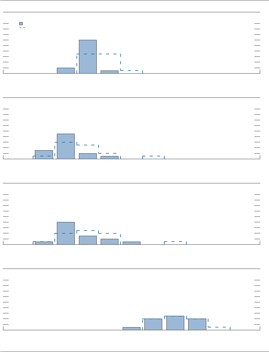
MONETARY POLICY REPORT: JULY 2018 53

Figure 3.B. Distribution of participants’ projections for the unemployment rate, 2018–20 and over the longer run

2018

Number of participants

3.0– 3.2– 3.4– 3.6– 3.8– 4.0– 4.2– 4.4– 4.6– 4.8– 5.0–

3.1 3.3 3.5 3.7 3.9 4.1 4.3 4.5 4.7 4.9 5.1

Percent range

June projections

March projections

2019

Number of participants

Percent range

2020

Number of participants

Percent range

Longer run

Number of participants

Percent range

N: Denitions of variables and other explanations are in the notes to table 1.

3.0– 3.2– 3.4– 3.6– 3.8– 4.0– 4.2– 4.4– 4.6– 4.8– 5.0–

3.1 3.3 3.5 3.7 3.9 4.1 4.3 4.5 4.7 4.9 5.1

3.0– 3.2– 3.4– 3.6– 3.8– 4.0– 4.2– 4.4– 4.6– 4.8– 5.0–

3.1 3.3 3.5 3.7 3.9 4.1 4.3 4.5 4.7 4.9 5.1

3.0– 3.2– 3.4– 3.6– 3.8– 4.0– 4.2– 4.4– 4.6– 4.8– 5.0–

3.1 3.3 3.5 3.7 3.9 4.1 4.3 4.5 4.7 4.9 5.1

54 PART 3: SUMMARY OF ECONOMIC PROJECTIONS

Figure 3.C. Distribution of participants’ projections for PCE ination, 2018–20 and over the longer run

2018

Number of participants

1.7– 1.9– 2.1– 2.3–

1.8 2.0 2.2 2.4

Percent range

June projections

March projections

2019

Number of participants

1.7– 1.9– 2.1– 2.3–

1.8 2.0 2.2 2.4

Percent range

2020

Number of participants

1.7– 1.9– 2.1– 2.3–

1.8 2.0 2.2 2.4

Percent range

Longer run

Number of participants

1.7– 1.9– 2.1– 2.3–

1.8 2.0 2.2 2.4

Percent range

N: Denitions of variables and other explanations are in the notes to table 1.

MONETARY POLICY REPORT: JULY 2018 55

Figure 3.D. Distribution of participants’ projections for core PCE ination, 2018–20

2018

Number of participants

1.7– 1.9– 2.1– 2.3–

1.8 2.0 2.2 2.4

Percent range

June projections

March projections

2019

Number of participants

1.7– 1.9– 2.1– 2.3–

1.8 2.0 2.2 2.4

Percent range

2020

Number of participants

1.7– 1.9– 2.1– 2.3–

1.8 2.0 2.2 2.4

Percent range

N: Denitions of variables and other explanations are in the notes to table 1.

56 PART 3: SUMMARY OF ECONOMIC PROJECTIONS

2018

Percent range

June projections

March projections

2019

Percent range

2020

Percent range

Longer run

Percent range

N: Denitions of variables and other explanations are in the notes to table 1.

Figure 3.E. Distribution of participants’ judgments of the midpoint of the appropriate target range for the federal

funds ra

te or the appropriate target level for the federal funds rate, 2018–20 and over the longer run

Number of participants

1.63–

1.87

1.88–

2.12

2.13–

2.37

2.38–

2.62

2.63–

2.87

2.88–

3.12

3.13–

3.37

3.38–

3.62

3.63–

3.87

3.88–

4.12

4.13–

4.37

4.38–

4.62

4.63–

4.87

4.88–

5.12

1.63–

1.87

1.88–

2.12

2.13–

2.37

2.38–

2.62

2.63–

2.87

2.88–

3.12

3.13–

3.37

3.38–

3.62

3.63–

3.87

3.88–

4.12

4.13–

4.37

4.38–

4.62

4.63–

4.87

4.88–

5.12

1.63–

1.87

1.88–

2.12

2.13–

2.37

2.38–

2.62

2.63–

2.87

2.88–

3.12

3.13–

3.37

3.38–

3.62

3.63–

3.87

3.88–

4.12

4.13–

4.37

4.38–

4.62

4.63–

4.87

4.88–

5.12

1.63–

1.87

1.88–

2.12

2.13–

2.37

2.38–

2.62

2.63–

2.87

2.88–

3.12

3.13–

3.37

3.38–

3.62

3.63–

3.87

3.88–

4.12

4.13–

4.37

4.38–

4.62

4.63–

4.87

4.88–

5.12

MONETARY POLICY REPORT: JULY 2018 57

graphically in the “fan charts” shown in

the top panels of gures 4.A, 4.B, and 4.C.

The fan charts display the median SEP

projections for the three variables surrounded

by symmetric condence intervals derived

from the forecast errors reported in table2.

If the degree of uncertainty attending these

projections is similar to the typical magnitude

of past forecast errors and the risks around the

projections are broadly balanced, then future

outcomes of these variables would have about

a 70percent probability of being within these

condence intervals. For all three variables,

this measure of uncertainty is substantial and

generally increases as the forecast horizon

lengthens.

Participants’ assessments of the level of

uncertainty surrounding their individual

economic projections are shown in the

bottom-left panels of gures4.A, 4.B,

and 4.C. Nearly all participants viewed

the degree of uncertainty attached to their

economic projections for real GDP growth,

the unemployment rate, and ination as

broadly similar to the average of the past

20years, a view that was essentially unchanged

from March.

Because the fan charts are constructed to be

symmetric around the median projections,

they do not reect any asymmetries in the

balance of risks that participants may see

in their economic projections. Participants’

assessments of the balance of risks to their

economic projections are shown in the

bottom-right panels of gures4.A, 4.B, and

4.C. Most participants judged the risks to

their projections of real GDP growth, the

unemployment rate, total ination, and core

ination as broadly balanced—in other words,

as broadly consistent with a symmetric fan

chart. Compared with March, even more

19. At the end of this summary, the box “Forecast

Uncertainty” discusses the sources and interpretation

of uncertainty surrounding the economic forecasts and

explains the approach used to assess the uncertainty and

risks attending the participants’ projections.

participants saw the risks to their projections

as broadly balanced. Specically, for GDP

growth, only one participant viewed the risks

as tilted to the downside, and the number of

participants who viewed the risks as tilted

to the upside dropped from four to two.

For the unemployment rate, the number of

participants who saw the risks as tilted toward

low readings dropped from four to two. For

ination, all but one participant judged the

risks to either total or core PCE price ination

as broadly balanced.

In discussing the uncertainty and risks

surrounding their projections, several

participants continued to point to scal

developments as a source of upside risk,

many participants cited developments related

to trade policy as posing downside risks to

their growth forecasts, and a few participants

also pointed to political developments in

Europe or the global outlook more generally

as downside-risk factors. A few participants

noted that the appreciation of the dollar

posed downside risks to the ination outlook.

A few participants also noted the risk of

ination moving higher than anticipated as the

unemployment rate falls.

Participants’ assessments of the appropriate

future path of the federal funds rate were also

subject to considerable uncertainty. Because

the Committee adjusts the federal funds

rate in response to actual and prospective

developments over time in real GDP growth,

the unemployment rate, and ination,

uncertainty surrounding the projected path

for the federal funds rate importantly reects

the uncertainties about the paths for those

key economic variables. Figure5 provides a

graphical representation of this uncertainty,

plotting the median SEP projection for the

federal funds rate surrounded by condence

intervals derived from the results presented

in table2. As with the macroeconomic

variables, forecast uncertainty surrounding the

appropriate path of the federal funds rate is

substantial and increases for longer horizons.

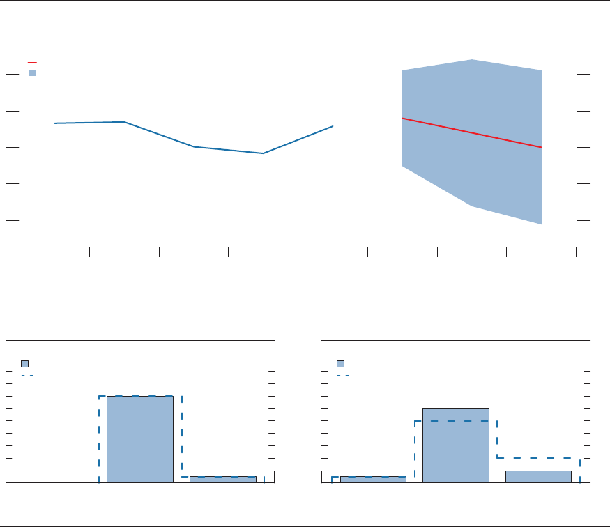
58 PART 3: SUMMARY OF ECONOMIC PROJECTIONS

Change in real GDP

Percent

2013 2014 2015 2016 2017 2018 2019 2020

Median of projections

70% condence interval

Actual

Number of participants

June projections

March projections

Risks to GDP growth

Number of participants

Weighted to

upside

Weighted to

downside

June projections

March projections

Figure 4.A. Uncertainty and risks in projections of GDP growth

Median projection and condence interval based on historical forecast errors

FOMC participants’ assessments of uncertainty and risks around their economic projections

Lower HigherBroadly

Similar

Broadly

balanced

Uncertainty about GDP growth

N

: The blue and red lines in the top panel show actual values and median projected values, respectively, of the percent change

in real gross domestic product (GDP) from the fourth quarter of the previous year to the fourth quarter of the year indicated. The

condence interval around the median projected values is assumed to be symmetric and is based on root mean

squared errors of

various private and government forecasts made over the previous 20 years; more information about these data is available in table 2.

Because current conditions may dier from those that prevailed, on average, over the previous 20 years, the width and shape of the

condence interval estimated on the basis of the historical forecast errors may not reect FOMC participants’ current assessments

of the uncertainty and risks around their projections; these current assessments are summarized in the lower panels. Generally

speaking, participants who judge the uncertainty about their projections as “broadly similar” to the average levels of the past

20 years would view the width of the condence interval shown in the historical fan chart as largely consistent with their assessments

of the uncertainty about their projections. Likewise, participants who judge the risks to their projections as “broadly balanced”

would view the condence interval around their projections as approximately symmetric. For denitions of uncertainty and risks in

economic projections, see the box “Forecast Uncertainty.”

MONETARY POLICY REPORT: JULY 2018 59

Figure 4.B. Uncertainty and risks in projections of the unemployment rate

Median projection and condence interval based on historical forecast errors

Unemployment rate

Percent

2013 2014 2015 2016 2017 2018 2019 2020

Median of projections

70% condence interval

Actual

FOMC participants’ assessments of uncertainty and risks around their economic projections

Uncertainty about the unemployment rate

June projections

March projections

Risks to the unemployment rate

June projections

March projections

Number of participants Number of participants

Weighted to

upside

Weighted to

downside

Lower HigherBroadly

Similar

Broadly

balanced

N: The blue and red lines in the top panel show actual values and median projected values, respectively, of the average

civilian unemployment rate in the fourth quarter of the year indicated. The condence interval around the median projected

values is assumed to be symmetric and is based on root mean squared errors of various private and government forecasts made

over the previous 20 years; more information about these data is available in table 2. Because current conditions may dier from

those that prevailed, on average, over the previous 20 years, the width and shape of the condence interval estimated on the basis

of the historical forecast errors may not reect FOMC participants’ current assessments of the uncertainty and risks around

their projections; these current assessments are summarized in the lower panels. Generally speaking, participants who judge the

uncertainty about their projections as “broadly similar” to the average levels of the past 20 years would view the width of the

condence interval shown in the historical fan chart as largely consistent with their assessments of the uncertainty about their

projections. Likewise, participants who judge the risks to their projections as “broadly balanced” would view the condence

interval around their projections as approximately symmetric. For denitions of uncertainty and risks in economic projections,

see the box “Forecast Uncertainty.”

60 PART 3: SUMMARY OF ECONOMIC PROJECTIONS

Figure 4.C. Uncertainty and risks in projections of PCE ination

Median projection and condence interval based on historical forecast errors

PCE ination

2013 2014 2015 2016 2017 2018 2019 2020

Median of projections

70% condence interval

Actual

FOMC participants’ assessments of uncertainty and risks around their economic projections

Uncertainty about PCE ination

June projections

March projections

Uncertainty about core PCE ination

Number of participants Number of participants

June projections

March projections

Risks to PCE ination

June projections

March projections

Risks to core PCE ination

June projections

March projections

Weighted to

upside

Weighted to

downside

Lower HigherBroadly

Similar

Broadly

balanced

Weighted to

upside

Weighted to

downside

Lower HigherBroadly

Similar

Broadly

balanced

Percent

: The blue and red lines in the top panel show actual values and median projected values, respectively, of the percent change

in the price inde

x for personal consumption expenditures (PCE) from the fourth quarter of the previous year to the fourth quarter

the year indicated. The condence interval around the median projected values is assumed to be symmetric and is based on root

mean squa

red errors of various private and government forecasts made over the previous 20 years; more information about these

ta is available in table 2. Because current conditions may dier from those that prevailed, on average, over the previous

20 years

, the width and shape of the condence interval estimated on the basis of the historical forecast errors may not reect

FOMC participants’

current assessments of the uncertainty and risks around their projections; these current assessments are

summariz

ed in the lower panels. Generally speaking, participants who judge the uncertainty about their projections as “broadly

similar”

to the average levels of the past 20 years would view the width of the condence interval shown in the historical fan

chart as lar

gely consistent with their assessments of the uncertainty about their projections. Likewise, participants who judge

the risks to their pr

ojections as “broadly balanced” would view the condence interval around their projections as approximately

symmetric. F

or denitions of uncertainty and risks in economic projections, see the box “Forecast Uncertainty.”

MONETARY POLICY REPORT: JULY 2018 61

Figure 5. Uncertainty in projections of the federal funds rate

Median projection and condence interval based on historical forecast errors

Federal funds rate

2013 2014 2015 2016 2017 2018 2019 2020

Midpoint of target range

Median of projections

70% condence interval*

Actual

Percent

: The blue and red lines are based on actual values and median projected values, respectively, of the Committee’s target for

the feder

al funds rate at the end of the year indicated. The actual values are the midpoint of the target range; the median projected

lues are based on either the midpoint of the target range or the target level. The condence interval around the median proje

cted

lues is based on root mean squared errors of various private and government forecasts made over the previous 20 years. The

condence interv

al is not strictly consistent with the projections for the federal funds rate, primarily because these projections are

not

forecasts of the likeliest outcomes for the federal funds rate, but rather projections of participants’ individual assessments of

ppropriate monetary policy. Still, historical forecast errors provide a broad sense of the uncertainty around the future path of the

feder

al funds rate generated by the uncertainty about the macroeconomic variables as well as additional adjustments to monetary

policy th

at may be appropriate to oset the eects of shocks to the economy.

The condence interval is assumed to be symmetric except when it is truncated at zero—the bottom of the lowest tar

get range

r the federal funds rate that has been adopted in the past by the Committee. This truncation would not be intended to indicat

the li

kelihood of the use of negative interest rates to provide additional monetary policy accommodation if

doing so was judged

ppropriate. In such situations, the Committee could also employ other tools, including forward guidance and large-scale asset

pur

chases, to provide additional accommodation. Because current conditions may dier from those that prevailed, on average,

er the previous 20 years, the width and shape of the condence interval estimated on the basis of the historical forecast errors

y not reect FOMC participants’ current assessments of the uncertainty and risks around their projections.

* The condence interval is derived from forecasts of the average level of short-term interest rates in the fourth quarter of

the year

indica

ted; more information about these data is available in table 2. The shaded area encompasses less than a 70 percent condence

interval if the condence interval has been truncated at zero.

62 PART 3: SUMMARY OF ECONOMIC PROJECTIONS

in the bottom-left panels of those gures. Participants

also provide judgments as to whether the risks to their

projections are weighted to the upside, are weighted to

the downside, or are broadly balanced. That is, while the

symmetric historical fan charts shown in the top panels of

gures4.A through 4.C imply that the risks to participants’

projections are balanced, participants may judge that

there is a greater risk that a given variable will be above

rather than below their projections. These judgments

are summarized in the lower-right panels of gures 4.A

through 4.C.

As with real activity and ination, the outlook for

the future path of the federal funds rate is subject to

considerable uncertainty. This uncertainty arises primarily

because each participant’s assessment of the appropriate

stance of monetary policy depends importantly on

the evolution of real activity and ination over time. If

economic conditions evolve in an unexpected manner,

then assessments of the appropriate setting of the federal

funds rate would change from that point forward. The

nal line in table2 shows the error ranges for forecasts of

short-term interest rates. They suggest that the historical

condence intervals associated with projections of the

federal funds rate are quite wide. It should be noted,

however, that these condence intervals are not strictly

consistent with the projections for the federal funds

rate, as these projections are not forecasts of the most

likely quarterly outcomes but rather are projections

of participants’ individual assessments of appropriate

monetary policy and are on an end-of-year basis.

However, the forecast errors should provide a sense of the

uncertainty around the future path of the federal funds rate

generated by the uncertainty about the macroeconomic

variables as well as additional adjustments to monetary

policy that would be appropriate to offset the effects of

shocks to the economy.

If at some point in the future the condence interval

around the federal funds rate were to extend below zero,

it would be truncated at zero for purposes of the fan chart

shown in gure5; zero is the bottom of the lowest target

range for the federal funds rate that has been adopted

by the Committee in the past. This approach to the

construction of the federal funds rate fan chart would be

merely a convention; it would not have any implications

for possible future policy decisions regarding the use of

negative interest rates to provide additional monetary

policy accommodation if doing so were appropriate. In

such situations, the Committee could also employ other

tools, including forward guidance and asset purchases, to

provide additional accommodation.

While gures 4.A through 4.C provide information on

the uncertainty around the economic projections, gure1

provides information on the range of views across FOMC

participants. A comparison of gure1 with gures4.A

through 4.C shows that the dispersion of the projections

across participants is much smaller than the average

forecast errors over the past 20years.

The economic projections provided by the members of

the Board of Governors and the presidents of the Federal

Reserve Banks inform discussions of monetary policy

among policymakers and can aid public understanding

of the basis for policy actions. Considerable uncertainty

attends these projections, however. The economic and

statistical models and relationships used to help produce

economic forecasts are necessarily imperfect descriptions

of the real world, and the future path of the economy

can be affected by myriad unforeseen developments and

events. Thus, in setting the stance of monetary policy,

participants consider not only what appears to be the

most likely economic outcome as embodied in their

projections, but also the range of alternative possibilities,

the likelihood of their occurring, and the potential costs to

the economy should they occur.

Table 2 summarizes the average historical accuracy

of a range of forecasts, including those reported in past

Monetary Policy Reports and those prepared by the

Federal Reserve Board’s staff in advance of meetings of the

Federal Open Market Committee (FOMC). The projection

error ranges shown in the table illustrate the considerable

uncertainty associated with economic forecasts. For

example, suppose a participant projects that real gross

domestic product (GDP) and total consumer prices will

rise steadily at annual rates of, respectively, 3percent and

2percent. If the uncertainty attending those projections

is similar to that experienced in the past and the risks

around the projections are broadly balanced, the numbers

reported in table2 would imply a probability of about

70percent that actual GDP would expand within a range

of 1.7 to 4.3percent in the current year, 1.0 to 5.0percent

in the second year, and 0.9 to 5.1percent in the third

year. The corresponding 70percent condence intervals

for overall ination would be 1.3 to 2.7percent in the

current year and 1.0 to 3.0percent in the second and third

years. Figures 4.A through 4.C illustrate these condence

bounds in “fan charts” that are symmetric and centered on

the medians of FOMC participants’ projections for GDP

growth, the unemployment rate, and ination. However,

in some instances, the risks around the projections may

not be symmetric. In particular, the unemployment rate

cannot be negative; furthermore, the risks around a

particular projection might be tilted to either the upside or

the downside, in which case the corresponding fan chart

would be asymmetrically positioned around the median

projection.

Because current conditions may differ from those that

prevailed, on average, over history, participants provide

judgments as to whether the uncertainty attached to

their projections of each economic variable is greater

than, smaller than, or broadly similar to typical levels

of forecast uncertainty seen in the past 20years, as

presented in table2 and reected in the widths of the

condence intervals shown in the top panels of gures

4.A through 4.C. Participants’ current assessments of the

uncertainty surrounding their projections are summarized

Forecast Uncertainty

AFE advanced foreign economy

BBA Bipartisan Budget Act of 2018

BLS Bureau of Labor Statistics

C&I commercial and industrial

Desk Open Market Desk at the Federal Reserve Bank of New York

DPI disposable personal income

ECB European Central Bank

EME emerging market economy

FOMC Federal Open Market Committee; also, the Committee

GDP gross domestic product

IOER interest on excess reserves

JOLTS Job Openings and Labor Turnover Survey

LFPR labor force participation rate

MBS mortgage-backed securities

Michigan survey University of Michigan Surveys of Consumers

OIS overnight index swap

ON RRP overnight reverse repurchase agreement

PCE personal consumption expenditures

SEP Summary of Economic Projections

SLOOS Senior Loan Ocer Opinion Survey on Bank Lending Practices

S&P Standard & Poor’s

TCJA Tax Cuts and Jobs Act

TIPS Treasury Ination-Protected Securities

VIX implied volatility for the S&P 500 index

abbreviations

Board of Governors of the Federal Reserve System

For use at 11:00 a.m., EDT

July 13, 2018

Monetary Policy rePort

July 13, 2018