
Contents
Preface vi
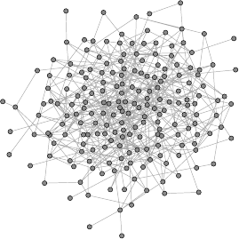
Appetizer: using probability to cover a geometric set 1
1 Preliminaries on random variables 5
1.1 Basic quantities associated with random variables 5
1.2 Some classical inequalities 6
1.3 Limit theorems 8
1.4 Notes 11
2 Concentration of sums of independent random variables 12
2.1 Why concentration inequalities? 12
2.2 Hoeffding’s inequality 15
2.3 Chernoff’s inequality 18
2.4 Application: degrees of random graphs 21
2.5 Sub-gaussian distributions 23
2.6 General Hoeffding’s and Khintchine’s inequalities 28
2.7 Sub-exponential distributions 31
2.8 Bernstein’s inequality 36
2.9 Notes 39
3 Random vectors in high dimensions 41
3.1 Concentration of the norm 42
3.2 Covariance matrices and principal component analysis 44
3.3 Examples of high-dimensional distributions 49
3.4 Sub-gaussian distributions in higher dimensions 55
3.5 Application: Grothendieck’s inequality and semidefinite programming 60
3.6 Application: Maximum cut for graphs 65
3.7 Kernel trick, and tightening of Grothendieck’s inequality 69
3.8 Notes 73
4 Random matrices 75
4.1 Preliminaries on matrices 75
4.2 Nets, covering numbers and packing numbers 80
4.3 Application: error correcting codes 85
4.4 Upper bounds on random sub-gaussian matrices 88
4.5 Application: community detection in networks 92
4.6 Two-sided bounds on sub-gaussian matrices 96
iii
iv Contents
4.7 Application: covariance estimation and clustering 99
4.8 Notes 102
5 Concentration without independence 104
5.1 Concentration of Lipschitz functions on the sphere 104
5.2 Concentration on other metric measure spaces 111
5.3 Application: Johnson-Lindenstrauss Lemma 117
5.4 Matrix Bernstein’s inequality 120
5.5 Application: community detection in sparse networks 128
5.6 Application: covariance estimation for general distributions 129
5.7 Notes 132
6 Quadratic forms, symmetrization and contraction 135
6.1 Decoupling 135
6.2 Hanson-Wright Inequality 139
6.3 Concentration of anisotropic random vectors 143
6.4 Symmetrization 145
6.5 Random matrices with non-i.i.d. entries 147
6.6 Application: matrix completion 149
6.7 Contraction Principle 152
6.8 Notes 155
7 Random processes 157
7.1 Basic concepts and examples 157
7.2 Slepian’s inequality 161
7.3 Sharp bounds on Gaussian matrices 168
7.4 Sudakov’s minoration inequality 171
7.5 Gaussian width 174
7.6 Stable dimension, stable rank, and Gaussian complexity 179
7.7 Random projections of sets 182
7.8 Notes 186
8 Chaining 189
8.1 Dudley’s inequality 189
8.2 Application: empirical processes 197
8.3 VC dimension 202
8.4 Application: statistical learning theory 215
8.5 Generic chaining 221
8.6 Talagrand’s majorizing measure and comparison theorems 225
8.7 Chevet’s inequality 227
8.8 Notes 229
9 Deviations of random matrices and geometric consequences 232
9.1 Matrix deviation inequality 232
9.2 Random matrices, random projections and covariance estimation 238
9.3 Johnson-Lindenstrauss Lemma for infinite sets 241
9.4 Random sections: M
∗
bound and Escape Theorem 244
9.5 Notes 248
Contents v
10 Sparse Recovery 250
10.1 High-dimensional signal recovery problems 250
10.2 Signal recovery based on M
∗
bound 252
10.3 Recovery of sparse signals 254
10.4 Low-rank matrix recovery 258
10.5 Exact recovery and the restricted isometry property 261
10.6 Lasso algorithm for sparse regression 267
10.7 Notes 271
11 Dvoretzky-Milman’s Theorem 273
11.1 Deviations of random matrices with respect to general norms 273
11.2 Johnson-Lindenstrauss embeddings and sharper Chevet inequality 277
11.3 Dvoretzky-Milman’s Theorem 278
11.4 Notes 283
Bibliography 284
Index 294

Preface
Who is this book for?
This is a textbook in probability in high dimensions with a view toward applica-
tions in data sciences. It is intended for doctoral and advanced masters students
and beginning researchers in mathematics, statistics, electrical engineering, com-
putational biology and related areas, who are looking to expand their knowledge
of theoretical methods used in modern research in data sciences.
Why this book?
Data sciences are moving fast, and probabilistic methods often provide a foun-
dation and inspiration for such advances. A typical graduate probability course
is no longer sufficient to acquire the level of mathematical sophistication that
is expected from a beginning researcher in data sciences today. The proposed
book intends to partially cover this gap. It presents some of the key probabilis-
tic methods and results that may form an essential toolbox for a mathematical
data scientist. This book can be used as a textbook for a basic second course in
probability with a view toward data science applications. It is also suitable for
self-study.
What is this book about?
High-dimensional probability is an area of probability theory that studies random
objects in R
n
where the dimension n can be very large. This book places par-
ticular emphasis on random vectors, random matrices, and random projections.
It teaches basic theoretical skills for the analysis of these objects, which include
concentration inequalities, covering and packing arguments, decoupling and sym-
metrization tricks, chaining and comparison techniques for stochastic processes,
combinatorial reasoning based on the VC dimension, and a lot more.
High-dimensional probability provides vital theoretical tools for applications
in data science. This book integrates theory with applications for covariance
estimation, semidefinite programming, networks, elements of statistical learning,
error correcting codes, clustering, matrix completion, dimension reduction, sparse
signal recovery, sparse regression, and more.
Prerequisites
The essential prerequisites for reading this book are a rigorous course in probabil-
ity theory (on Masters or Ph.D. level), an excellent command of undergraduate
linear algebra, and general familiarity with basic notions about metric, normed
vi
Preface vii
and Hilbert spaces and linear operators. Knowledge of measure theory is not
essential but would be helpful.
A word on exercises
Exercises are integrated into the text. The reader can do them immediately to
check his or her understanding of the material just presented, and to prepare
better for later developments. The difficulty of the exercises is indicated by the
number of coffee cups; it can range from easiest (K) to hardest (KKKK).
Related reading
This book covers only a fraction of theoretical apparatus of high-dimensional
probability, and it illustrates it with only a sample of data science applications.
Each chapter in this book is concluded with a Notes section, which has pointers
to other texts on the matter. A few particularly useful sources should be noted
here. The now classical book [8] showcases the probabilistic method in applica-
tions to discrete mathematics and computer science. The forthcoming book [20]
presents a panorama of mathematical data science, and it particularly focuses
on applications in computer science. Both these books are accessible to gradu-
ate and advanced undergraduate students. The lecture notes [212] are pitched
for graduate students and present more theoretical material in high-dimensional
probability.
Acknowledgements
The feedback from my many colleagues was instrumental in perfecting this book.
My thanks go to Florent Benaych-Georges, Jennifer Bryson, Lukas Gr¨atz, Remi
Gribonval, Ping Hsu, Mike Izbicki, Yi Li, George Linderman, Cong Ma, Galyna
Livshyts, Jelani Nelson, Ekkehard Schnoor, Martin Spindler, Dominik St¨oger,
Tim Sullivan, Terence Tao, Joel Tropp, Katarzyna Wyczesany, Yifei Shen and
Haoshu Xu for many valuable suggestions and corrections, especially to Sjoerd
Dirksen, Larry Goldstein, Wu Han, Han Wu, and Mahdi Soltanolkotabi for de-
tailed proofreading of the book, Can Le, Jennifer Bryson and my son Ivan Ver-
shynin for their help with many pictures in this book.
After this book had been published, many colleagues offered further sugges-
tions and noticed many typos, gaps and inaccuracies. I am grateful to Karthik
Abinav, Diego Armentano, Aaron Berk, Soham De, Hu Fu, Adam Jozefiak, Nick
Harvey, Harrie Hendriks, Joris K¨uhl, Jana Kr¨agel, Yi Li, Chris Liaw, Hengrui
Luo, Pete Morcos, Adrien Peltzer, Sikander Randhawa, Karthik Sankararaman,
Nils Siebken, Morten Thonack, and especially to Franz Haniel, Ichiro Hashimoto,
Aryeh Kontorovich, Jake Knigge, Wai-Kit Lam, Yi Li, Mark Meckes, Abbas
Mehrabian, Holger Rauhut, Michael Scheutzow, and Hao Xing who offered sub-
stantial feedback that lead to significant improvements.
The issues that are found after publication have been corrected in the electronic
version. Please feel free to send me any further feedback.
Irvine, California
May 20, 2024

Appetizer: using probability to cover a geometric set
We begin our study of high-dimensional probability with an elegant argument
that showcases the usefulness of probabilistic reasoning in geometry.
Recall that a convex combination of points z
1
, . . . , z
m
∈ R
n
is a linear combi-
nation with coefficients that are non-negative and sum to 1, i.e. it is a sum of the
form
m
X
i=1
λ
i
z
i
where λ
i
≥ 0 and
m
X
i=1
λ
i
= 1. (0.1)
The convex hull of a set T ⊂ R
n
is the set of all convex combinations of all finite
collections of points in T :
conv(T )
:
= {convex combinations of z
1
, . . . , z
m
∈ T for m ∈ N};
see Figure 0.1 for illustration.
Figure 0.1 The convex hull of a set of points representing major U.S. cities
The number m of elements defining a convex combination in R
n
is not restricted
a priori. However, the classical Caratheodory’s theorem states that one can always
take m ≤ n + 1.
Theorem 0.0.1 (Caratheodory’s theorem). Every point in the convex hull of a
set T ⊂ R
n
can be expressed as a convex combination of at most n + 1 points
from T .
The bound n + 1 can not be improved, as it is clearly attained for a simplex T
(a set of n + 1 points in general position). Suppose, however, that we only want
1

2 Appetizer: using probability to cover a geometric set
to approximate a point x ∈ conv(T ) rather than exactly represent it as a convex
combination. Can we do it with fewer than n + 1 points? We now show that this
is possible, and actually the number of required points does not need to depend
on the dimension n at all!
Theorem 0.0.2 (Approximate Caratheodory’s theorem). Consider a set T ⊂ R
n
whose diameter
1
is bounded by 1. Then, for every point x ∈ conv(T ) and every
integer k, one can find points x
1
, . . . , x
k
∈ T such that
x −
1
k
k
X
j=1
x
j
2
≤
1
√
k
.
There are two reasons why this result is surprising. First, the number of points
k in convex combinations does not depend on the dimension n. Second, the co-
efficients of convex combinations can be made all equal. (Note however that
repetitions among the points x
i
are allowed.)
Proof Our argument is known as the empirical method of B. Maurey.
Translating T if necessary, we may assume that not only the diameter but also
the radius of T is bounded by 1, i.e.
∥t∥
2
≤ 1 for all t ∈ T. (0.2)
Fix a point x ∈ conv(T ) and express it as a convex combination of some vectors
z
1
, . . . , z
m
∈ T as in (0.1). Now, interpret the definition of convex combination
(0.1) probabilistically, with λ
i
taking the roles of probabilities. Specifically, we
can define a random vector Z that takes values z
i
with probabilities λ
i
:
P
Z = z
i
= λ
i
, i = 1, . . . , m.
(This is possible by the fact that the weights λ
i
are non-negative and sum to
one.) Then
E Z =
m
X
i=1
λ
i
z
i
= x.
Consider independent copies Z
1
, Z
2
, . . . of Z. By the the strong law of large
numbers,
1
k
k
X
j=1
Z
j
→ x almost surely as k → ∞.
To get a quantitative form of this result, let us compute the variance of
1
k
P
k
j=1
Z
j
.
(Incidentally, this computation is at the heart of the proof of the weak law of large
numbers). We obtain
E
x −
1
k
k
X
j=1
Z
j
2
2
=
1
k
2
E
k
X
j=1
(Z
j
− x)
2
2
=
1
k
2
k
X
j=1
E ∥Z
j
− x∥
2
2
1
The diameter of T is defined as diam(T ) = sup{∥s − t∥
2
:
s, t ∈ T }. We assumed that diam(T ) = 1
for simplicity. For a general set T , the bound in the theorem changes to diam(T )/
√
k. Check this!

Appetizer: using probability to cover a geometric set 3
since E(Z
i
−x) = 0 for each i. The last identity is just a higher dimensional version
of the basic fact that the variance of a sum of independent random variables equals
the sum of variances; see Exercise 0.0.3 below.
It remains to bound the variances of the terms. We have
E∥Z
j
− x∥
2
2
= E ∥Z − E Z∥
2
2
= E ∥Z∥
2
2
− ∥E Z∥
2
2
(another variance identity; see Exercise 0.0.3)
≤ E ∥Z∥
2
2
≤ 1 (since Z ∈ T and using (0.2)).
We showed that
E
x −
1
k
k
X
j=1
Z
j
2
2
≤
1
k
.
Therefore, there exists a realization of the random variables Z
1
, . . . , Z
k
such that
x −
1
k
k
X
j=1
Z
j
2
2
≤
1
k
.
Since by construction each Z
j
takes values in T , the proof is complete.
Exercise 0.0.3. KK Check the following variance identities that we used in
the proof of Theorem 0.0.2.
(a) Let Z
1
, . . . , Z
k
be independent mean zero random vectors in R
n
. Show that
E
k
X
j=1
Z
j
2
2
=
k
X
j=1
E ∥Z
j
∥
2
2
.
(b) Let Z be a random vector in R
n
. Show that
E ∥Z − E Z∥
2
2
= E ∥Z∥
2
2
− ∥E Z∥
2
2
.
Let us give one application of Theorem 0.0.2 in computational geometry. Sup-
pose we are given a subset P ⊂ R
n
and ask to cover it by balls of given radius
ε, see Figure 0.2. What is the smallest number of balls needed, and how shall we
place them?
Figure 0.2 The covering problem asks how many balls of radius ε are
needed to cover a given set in R
n
, and where to place these balls.

4 Appetizer: using probability to cover a geometric set
Corollary 0.0.4 (Covering polytopes by balls). Let P be a polytope in R
n
with
N vertices and whose diameter is bounded by 1. Then P can be covered by at
most N
⌈1/ε
2
⌉
Euclidean balls of radii ε > 0.
Proof Let us define the centers of the balls as follows. Let k
:
= ⌈1/ε
2
⌉ and
consider the set
N
:
=
1
k
k
X
j=1
x
j
:
x
j
are vertices of P
.
We claim that the family of ε-balls centered at N satisfy the conclusion of the
corollary. To check this, note that the polytope P is the convex hull of the set
of its vertices, which we denote by T . Thus we can apply Theorem 0.0.2 to any
point x ∈ P = conv(T ) and deduce that x is within distance 1/
√
k ≤ ε from
some point in N. This shows that the ε-balls centered at N indeed cover P .
To bound the cardinality of N, note that there are N
k
ways to choose k out of
N vertices with repetition. Thus |N| ≤ N
k
= N
⌈1/ε
2
⌉
. The proof is complete.
In this book we learn several other approaches to the covering problem when we
relate it to packing (Section 4.2), entropy and coding (Section 4.3) and random
processes (Chapters 7–8).
To finish this section, let us show how to slightly improve Corollary 0.0.4.
Exercise 0.0.5 (The sum of binomial coefficients). KK Prove the inequalities
n
m
m
≤
n
m
!
≤
m
X
k=0
n
k
!
≤
en
m
m
for all integers m ∈ [1, n].
Hint: To prove the upper bound, multiply both sides by the quantity (m/n)
m
, replace this quantity by
(m/n)
k
in the left side, and use the Binomial Theorem.
Exercise 0.0.6 (Improved covering). KK Check that in Corollary 0.0.4,
(C + Cε
2
N)
⌈1/ε
2
⌉
suffice. Here C is a suitable absolute constant. (Note that this bound is slightly
stronger than N
⌈1/ε
2
⌉
for small ε.)
Hint: The number of ways to choose an (unordered) subset of k elements from an N-element set with
repetition is
N+k−1
k
. Simplify using Exercise 0.0.5.
0.0.1 Notes
In this section we gave an illustration of the probabilistic method, where one
employs randomness to construct a useful object. The book [8] presents many
illustrations of the probabilistic method, mainly in combinatorics.
The empirical method of B. Maurey we presented in this section was originally
proposed in [166]. B. Carl used it to get bounds on covering numbers [49] including
those stated in Corollary 0.0.4 and Exercise 0.0.6. The bound in Exercise 0.0.6 is
sharp [49, 50].

1
Preliminaries on random variables
In this chapter we recall some basic concepts and results of probability theory. The
reader should already be familiar with most of this material, which is routinely
taught in introductory probability courses.
Expectation, variance, and moments of random variables are introduced in
Section 1.1. Some classical inequalities can be found in Section 1.2. The two
fundamental limit theorems of probability – the law of large numbers and the
central limit theorem – are recalled in Section 1.3.
1.1 Basic quantities associated with random variables
In a basic course in probability theory, we learned about the two most important
quantities associated with a random variable X, namely the expectation
1
(also
called mean), and variance. They will be denoted in this book by
2
E X and Var(X) = E(X − E X)
2
.
Let us recall some other classical quantities and functions that describe prob-
ability distributions. The moment generating function of X is defined as
M
X
(t) = E e
tX
, t ∈ R.
For p > 0, the p-th moment of X is defined as E X
p
, and the p-th absolute moment
is E |X|
p
.
It is useful to take p-th root of the moments, which leads to the notion of the
L
p
norm of a random variable:
∥X∥
L
p
= (E |X|
p
)
1/p
, p ∈ (0, ∞).
This definition can be extended to p = ∞ by the essential supremum of |X|:
∥X∥
L
∞
= ess sup |X|.
For fixed p and a given probability space (Ω, Σ, P), the classical vector space
1
If you studied measure theory, you will recall that the expectation E X of a random variable X on a
probability space (Ω, Σ, P) is, by definition, the Lebesgue integral of the function X
:
Ω → R. This
makes all theorems on Lebesgue integration applicable in probability theory, for expectations of
random variables.
2
Throughout this book, we drop the brackets in the notation E[f (X)] and simply write E f(X)
instead. Thus, nonlinear functions bind before expectation.
5

6 Preliminaries
L
p
= L
p
(Ω, Σ, P) consists of all random variables X on Ω with finite L
p
norm,
that is
L
p
=
n
X
:
∥X∥
L
p
< ∞
o
.
If p ∈ [1, ∞], the quantity ∥X∥
L
p
is a norm and L
p
is a Banach space. This
fact follows from Minkowski’s inequality, which we recall in (1.4). For p < 1, the
triangle inequality fails and ∥X∥
L
p
is not a norm.
The exponent p = 2 is special in that L
2
is not only a Banach space but also a
Hilbert space. The inner product and the corresponding norm on L
2
are given by
⟨X, Y ⟩
L
2
= E XY, ∥X∥
L
2
= (E |X|
2
)
1/2
. (1.1)
Then the standard deviation of X can be expressed as
∥X − E X∥
L
2
=
q
Var(X) = σ(X).
Similarly, we can express the covariance of random variables of X and Y as
cov(X, Y ) = E(X − E X)(Y − E Y ) = ⟨X − E X, Y − E Y ⟩
L
2
. (1.2)
Remark 1.1.1 (Geometry of random variables). When we consider random vari-
ables as vectors in the Hilbert space L
2
, the identity (1.2) gives a geometric inter-
pretation of the notion of covariance. The more the vectors X −E X and Y −E Y
are aligned with each other, the bigger their inner product and covariance are.
1.2 Some classical inequalities
Jensen’s inequality states that for any random variable X and a convex
3
function
φ
:
R → R, we have
φ(E X) ≤ E φ(X).
As a simple consequence of Jensen’s inequality, ∥X∥
L
p
is an increasing function
in p, that is
∥X∥
L
p
≤ ∥X∥
L
q
for any 0 ≤ p ≤ q ≤ ∞. (1.3)
This inequality follows since ϕ(x) = x
q/p
is a convex function if q/p ≥ 1.
Minkowski’s inequality states that for any p ∈ [1, ∞] and any random variables
X, Y ∈ L
p
, we have
∥X + Y ∥
L
p
≤ ∥X∥
L
p
+ ∥Y ∥
L
p
. (1.4)
This can be viewed as the triangle inequality, which implies that ∥·∥
L
p
is a norm
when p ∈ [1, ∞].
The Cauchy-Schwarz inequality states that for any random variables X, Y ∈ L
2
,
we have
|E XY | ≤ ∥X∥
L
2
∥Y ∥
L
2
.
3
By definition, a function φ is convex if φ(λx + (1 − λ)y) ≤ λφ(x) + (1 − λ)φ(y) for all t ∈ [0, 1] and
all vectors x, y in the domain of φ.

1.2 Some classical inequalities 7
The more general H¨older’s inequality states that if p, q ∈ (1, ∞) are conjugate
exponents, that is 1/p + 1/q = 1, then the random variables X ∈ L
p
and Y ∈ L
q
satisfy
|E XY | ≤ ∥X∥
L
p
∥Y ∥
L
q
.
This inequality also holds for the pair p = 1, q = ∞.
As we recall from a basic probability course, the distribution of a random vari-
able X is, intuitively, the information about what values X takes with what
probabilities. More rigorously, the distribution of X is determined by the cumu-
lative distribution function (CDF) of X, defined as
F
X
(t) = P
X ≤ t
, t ∈ R.
It is often more convenient to work with tails of random variables, namely with
P
X > t
= 1 − F
X
(t).
There is an important connection between the tails and the expectation (and
more generally, the moments) of a random variable. The following identity is
typically used to bound the expectation by tails.
Lemma 1.2.1 (Integral identity). Let X be a non-negative random variable.
Then
E X =
Z
∞
0
P
X > t
dt.
The two sides of this identity are either finite or infinite simultaneously.
Proof We can represent any non-negative real number x via the identity
4
x =
Z
x
0
1 dt =
Z
∞
0
1
{t<x}
dt.
Substitute the random variable X for x and take expectation of both sides. This
gives
E X = E
Z
∞
0
1
{t<X}
dt =
Z
∞
0
E 1
{t<X}
dt =
Z
∞
0
P
t < X
dt.
To change the order of expectation and integration in the second equality, we
used Fubini-Tonelli’s theorem. The proof is complete.
Exercise 1.2.2 (Generalization of integral identity). K Prove the following ex-
tension of Lemma 1.2.1, which is valid for any random variable X (not necessarily
non-negative):
E X =
Z
∞
0
P
X > t
dt −
Z
0
−∞
P
X < t
dt.
4
Here and later in this book, 1
E
denotes the indicator of the event E, which is the function that
takes value 1 if E occurs and 0 otherwise.

8 Preliminaries
Exercise 1.2.3 (p-moments via tails). K Let X be a random variable and
p ∈ (0, ∞). Show that
E |X|
p
=
Z
∞
0
pt
p−1
P
|X| > t
dt
whenever the right hand side is finite.
Hint: Use the integral identity for |X|
p
and change variables.
Another classical tool, Markov’s inequality, can be used to bound the tail in
terms of expectation.
Proposition 1.2.4 (Markov’s Inequality). For any non-negative random variable
X and t > 0, we have
P
X ≥ t
≤
E X
t
.
Proof Fix t > 0. We can represent any real number x via the identity
x = x1
{x≥t}
+ x1
{x<t}
.
Substitute the random variable X for x and take expectation of both sides. This
gives
E X = E X1
{X≥t}
+ E X1
{X<t}
≥ E t1
{X≥t}
+ 0 = t · P
X ≥ t
.
Dividing both sides by t, we complete the proof.
A well-known consequence of Markov’s inequality is the following Chebyshev’s
inequality. It offers a better, quadratic dependence on t, and instead of the plain
tails, it quantifies the concentration of X about its mean.
Corollary 1.2.5 (Chebyshev’s inequality). Let X be a random variable with
mean µ and variance σ
2
. Then, for any t > 0, we have
P
|X − µ| ≥ t
≤
σ
2
t
2
.
Exercise 1.2.6. K Deduce Chebyshev’s inequality by squaring both sides of
the bound |X − µ| ≥ t and applying Markov’s inequality.
Remark 1.2.7. In Proposition 2.5.2 we will establish relations among the three
basic quantities associated with random variables – the moment generating func-
tions, the L
p
norms, and the tails.
1.3 Limit theorems
The study of sums of independent random variables forms core of the classical
probability theory. Recall that the identity
Var(X
1
+ ··· + X
N
) = Var(X
1
) + ··· + Var(X
N
)

1.3 LLN and CLT 9
holds for any independent random variables X
1
, . . . , X
N
. If, furthermore, X
i
have
the same distribution with mean µ and variance σ
2
, then dividing both sides by
N
2
we see that
Var
1
N
N
X
i=1
X
i
=
σ
2
N
. (1.5)
Thus, the variance of the sample mean
1
N
P
N
i=1
X
i
of the sample of {X
1
, . . . , X
N
}
shrinks to zero as N → ∞. This indicates that for large N, we should expect
that the sample mean concentrates tightly about its expectation µ. One of the
most important results in probability theory – the law of large numbers – states
precisely this.
Theorem 1.3.1 (Strong law of large numbers). Let X
1
, X
2
, . . . be a sequence of
i.i.d. random variables with mean µ. Consider the sum
S
N
= X
1
+ ···X
N
.
Then, as N → ∞,
S
N
N
→ µ almost surely.
The next result, the central limit theorem, makes one step further. It identifies
the limiting distribution of the (properly scaled) sum of X
i
’s as the normal dis-
tribution, sometimes also called Gaussian distribution. Recall that the standard
normal distribution, denoted N(0, 1), has density
f(x) =
1
√
2π
e
−x
2
/2
, x ∈ R. (1.6)
Theorem 1.3.2 (Lindeberg-L´evy central limit theorem). Let X
1
, X
2
, . . . be a
sequence of i.i.d. random variables with mean µ and variance σ
2
. Consider the
sum
S
N
= X
1
+ ··· + X
N
and normalize it to obtain a random variable with zero mean and unit variance
as follows:
Z
N
:
=
S
N
− E S
N
p
Var(S
N
)
=
1
σ
√
N
N
X
i=1
(X
i
− µ).
Then, as N → ∞,
Z
N
→ N(0, 1) in distribution.
The convergence in distribution means that the CDF of the normalized sum
converges pointwise to the CDF of the standard normal distribution. We can
express this in terms of tails as follows. Then for every t ∈ R, we have
P
Z
N
≥ t
→ P
g ≥ t
=
1
√
2π
Z
∞
t
e
−x
2
/2
dx
as N → ∞, where g ∼ N(0, 1) is a standard normal random variable.

10 Preliminaries
Exercise 1.3.3. K Let X
1
, X
2
, . . . be a sequence of i.i.d. random variables with
mean µ and finite variance. Show that
E
1
N
N
X
i=1
X
i
− µ
= O
1
√
N
as N → ∞.
One remarkable special case of the central limit theorem is where X
i
are
Bernoulli random variables with some fixed parameter p ∈ (0, 1), denoted
X
i
∼ Ber(p).
Recall that this means that X
i
take values 1 and 0 with probabilities p and 1 −p
respectively; also recall that E X
i
= p and Var(X
i
) = p(1 − p). The sum
S
N
:
= X
1
+ ··· + X
N
is said to have the binomial distribution Binom(N, p). The central limit theorem
(Theorem 1.3.2) yields that as N → ∞,
S
N
− Np
p
Np(1 − p)
→ N(0, 1) in distribution. (1.7)
This special case of the central limit theorem is called de Moivre-Laplace theorem.
Now suppose that X
i
∼ Ber(p
i
) with parameters p
i
that decay to zero as
N → ∞ so fast that the sum S
N
has mean O(1) instead of being proportional to
N. The central limit theorem fails in this regime. A different result we are about
to state says that S
N
still converges, but to the Poisson instead of the normal
distribution.
Recall that a random variable Z has Poisson distribution with parameter λ,
denoted
Z ∼ Pois(λ),
if it takes values in {0, 1, 2, . . .} with probabilities
P
Z = k
= e
−λ
λ
k
k!
, k = 0, 1, 2, . . . (1.8)
Theorem 1.3.4 (Poisson Limit Theorem). Let X
N,i
, 1 ≤ i ≤ N, be independent
random variables X
N,i
∼ Ber(p
N,i
), and let S
N
=
P
N
i=1
X
N,i
. Assume that, as
N → ∞,
max
i≤N
p
N,i
→ 0 and E S
N
=
N
X
i=1
p
N,i
→ λ < ∞.
Then, as N → ∞,
S
N
→ Pois(λ) in distribution.
1.4 Notes 11
1.4 Notes
The material presented in this chapter is included in most graduate probabil-
ity textbooks. In particular, proofs of the strong law of large numbers (Theo-
rem 1.3.1) and Lindeberg-L´evy central limit theorem (Theorem 1.3.2) can be
found e.g. in [72, Sections 1.7 and 2.4] and [23, Sections 6 and 27].
Both Proposition 1.2.4 and Corollary 1.2.5 are due to Chebyshev. However,
following the established tradition, we call Proposition 1.2.4 Markov’s inequality.

2
Concentration of sums of independent
random variables
This chapter introduces the reader to the rich topic of concentration inequalities.
After motivating the subject in Section 2.1, we prove some basic concentration
inequalities: Hoeffding’s in Sections 2.2 and 2.6, Chernoff’s in Section 2.3 and
Bernstein’s in Section 2.8. Another goal of this chapter is to introduce two im-
portant classes of distributions: sub-gaussian in Section 2.5 and sub-exponential
in Section 2.7. These classes form a natural “habitat” in which many results
of high-dimensional probability and its applications will be developed. We give
two quick applications of concentration inequalities for randomized algorithms in
Section 2.2 and random graphs in Section 2.4. Many more applications are given
later in the book.
2.1 Why concentration inequalities?
Concentration inequalities quantify how a random variable X deviates around its
mean µ. They usually take the form of two-sided bounds for the tails of X − µ,
such as
P
|X − µ| > t
≤ something small.
The simplest concentration inequality is Chebyshev’s inequality (Corollary 1.2.5).
It is very general but often too weak. Let us illustrate this with the example of
the binomial distribution.
Question 2.1.1. Toss a fair coin N times. What is the probability that we get
at least
3
4
N heads?
Let S
N
denote the number of heads. Then
E S
N
=
N
2
, Var(S
N
) =
N
4
.
Chebyshev’s inequality bounds the probability of getting at least
3
4
N heads as
follows:
P
S
N
≥
3
4
N
≤ P
(
S
N
−
N
2
≥
N
4
)
≤
4
N
. (2.1)
So the probability converges to zero at least linearly in N .
12

2.1 Why concentration inequalities? 13
Is this the right rate of decay, or we should expect something faster? Let us ap-
proach the same question using the central limit theorem. To do this, we represent
S
N
as a sum of independent random variables:
S
N
=
N
X
i=1
X
i
where X
i
are independent Bernoulli random variables with parameter 1/2, i.e.
P
X
i
= 0
= P
X
i
= 1
= 1/2. (These X
i
are the indicators of heads.) De
Moivre-Laplace central limit theorem (1.7) states that the distribution of the
normalized number of heads
Z
N
=
S
N
− N/2
p
N/4
converges to the standard normal distribution N(0, 1). Thus we should anticipate
that for large N, we have
P
S
N
≥
3
4
N
= P
Z
N
≥
q
N/4
≈ P
g ≥
q
N/4
(2.2)
where g ∼ N(0, 1). To understand how this quantity decays in N, we now get a
good bound on the tails of the normal distribution.
Proposition 2.1.2 (Tails of the normal distribution). Let g ∼ N(0, 1). Then for
all t > 0, we have
1
t
−
1
t
3
·
1
√
2π
e
−t
2
/2
≤ P
g ≥ t
≤
1
t
·
1
√
2π
e
−t
2
/2
In particular, for t ≥ 1 the tail is bounded by the density:
P
g ≥ t
≤
1
√
2π
e
−t
2
/2
. (2.3)
Proof To obtain an upper bound on the tail
P
g ≥ t
=
1
√
2π
Z
∞
t
e
−x
2
/2
dx,
let us change variables x = t + y. This gives
P
g ≥ t
=
1
√
2π
Z
∞
0
e
−t
2
/2
e
−ty
e
−y
2
/2
dy ≤
1
√
2π
e
−t
2
/2
Z
∞
0
e
−ty
dy,
where we used that e
−y
2
/2
≤ 1. Since the last integral equals 1/t, the desired
upper bound on the tail follows.
The lower bound follows from the identity
Z
∞
t
(1 − 3x
−4
)e
−x
2
/2
dx =
1
t
−
1
t
3
e
−t
2
/2
.
This completes the proof.

14 Sums of independent random variables
Returning to (2.2), we see that we should expect the probability of having at
least
3
4
N heads to be smaller than
1
√
2π
e
−N/8
. (2.4)
This quantity decays to zero exponentially fast in N, which is much better than
the linear decay in (2.1) that follows from Chebyshev’s inequality.
Unfortunately, (2.4) does not follow rigorously from the central limit theorem.
Although the approximation by the normal density in (2.2) is valid, the error
of approximation can not be ignored. And, unfortunately, the error decays too
slow – even slower than linearly in N. This can be seen from the following sharp
quantitative version of the central limit theorem.
Theorem 2.1.3 (Berry-Esseen central limit theorem). In the setting of Theo-
rem 1.3.2, for every N and every t ∈ R we have
P
Z
N
≥ t
− P
g ≥ t
≤
ρ
√
N
.
Here ρ = E |X
1
− µ|
3
/σ
3
and g ∼ N(0, 1).
Thus the approximation error in (2.2) is of order 1/
√
N, which ruins the desired
exponential decay (2.4).
Can we improve the approximation error in central limit theorem? In general,
no. If N is even, then the probability of getting exactly N/2 heads is
P
S
N
= N/2
= 2
−N
N
N/2
!
≍
1
√
N
;
the last estimate can be obtained using Stirling’s approximation.
1
(Do it!) Hence,
P
Z
N
= 0
≍ 1/
√
N. On the other hand, since the normal distribution is con-
tinuous, we have P
g = 0
= 0. Thus the approximation error here has to be of
order 1/
√
N.
Let us summarize our situation. The Central Limit theorem offers an approx-
imation of a sum of independent random variables S
N
= X
1
+ . . . + X
N
by the
normal distribution. The normal distribution is especially nice due to its very
light, exponentially decaying tails. At the same time, the error of approxima-
tion in central limit theorem decays too slow, even slower than linear. This big
error is a roadblock toward proving concentration properties for S
N
with light,
exponentially decaying tails.
In order to resolve this issue, we develop alternative, direct approaches to
concentration, which bypass the central limit theorem.
1
Our somewhat informal notation f ≍ g stands for the equivalence of functions (functions of N in
this particular example) up to constant factors. Precisely, f ≍ g means that there exist positive
constants c, C such that the inequality cf (x) ≤ g(x) ≤ Cf(x) holds for all x, or sometimes for all
sufficiently large x. For similar one-sided inequalities that hold up to constant factors, we use
notation f ≲ g and f ≳ g.

2.2 Hoeffding’s inequality 15
Exercise 2.1.4 (Truncated normal distribution). K Let g ∼ N(0, 1). Show
that for all t ≥ 1, we have
E g
2
1
{g>t}
= t ·
1
√
2π
e
−t
2
/2
+ P
g > t
≤
t +
1
t
1
√
2π
e
−t
2
/2
.
Hint: Integrate by parts.
2.2 Hoeffding’s inequality
We start with a particularly simple concentration inequality, which holds for sums
of i.i.d. symmetric Bernoulli random variables.
Definition 2.2.1 (Symmetric Bernoulli distribution). A random variable X has
symmetric Bernoulli distribution (also called Rademacher distribution) if it takes
values −1 and 1 with probabilities 1/2 each, i.e.
P
X = −1
= P
X = 1
=
1
2
.
Clearly, a random variable X has the (usual) Bernoulli distribution with pa-
rameter 1/2 if and only if Z = 2X − 1 has symmetric Bernoulli distribution.
Theorem 2.2.2 (Hoeffding’s inequality). Let X
1
, . . . , X
N
be independent sym-
metric Bernoulli random variables, and a = (a
1
, . . . , a
N
) ∈ R
N
. Then, for any
t ≥ 0, we have
P
N
X
i=1
a
i
X
i
≥ t
≤ exp
−
t
2
2∥a∥
2
2
!
.
Proof We can assume without loss of generality that ∥a∥
2
= 1. (Why?)
Let us recall how we deduced Chebyshev’s inequality (Corollary 1.2.5): we
squared both sides and applied Markov’s inequality. Let us do something similar
here. But instead of squaring both sides, let us multiply by a fixed parameter
λ > 0 (to be chosen later) and exponentiate. This gives
P
N
X
i=1
a
i
X
i
≥ t
= P
exp
λ
N
X
i=1
a
i
X
i
≥ exp(λt)
≤ e
−λt
E exp
λ
N
X
i=1
a
i
X
i
. (2.5)
In the last step we applied Markov’s inequality (Proposition 1.2.4).
We thus reduced the problem to bounding the moment generating function
(MGF) of the sum
P
N
i=1
a
i
X
i
. As we recall from a basic probability course, the
MGF of the sum is the product of the MGF’s of the terms; this follows immedi-
ately from independence. Thus
E exp
λ
N
X
i=1
a
i
X
i
=
N
Y
i=1
E exp(λa
i
X
i
). (2.6)

16 Sums of independent random variables
Let us fix i. Since X
i
takes values −1 and 1 with probabilities 1/2 each, we
have
E exp(λa
i
X
i
) =
exp(λa
i
) + exp(−λa
i
)
2
= cosh(λa
i
).
Exercise 2.2.3 (Bounding the hyperbolic cosine). K Show that
cosh(x) ≤ exp(x
2
/2) for all x ∈ R.
Hint: Compare the Taylor’s expansions of both sides.
This bound shows that
E exp(λa
i
X
i
) ≤ exp(λ
2
a
2
i
/2).
Substituting into (2.6) and then into (2.5), we obtain
P
N
X
i=1
a
i
X
i
≥ t
≤ e
−λt
N
Y
i=1
exp(λ
2
a
2
i
/2) = exp
− λt +
λ
2
2
N
X
i=1
a
2
i
= exp
− λt +
λ
2
2
.
In the last identity, we used the assumption that ∥a∥
2
= 1.
This bound holds for arbitrary λ > 0. It remains to optimize in λ; the minimum
is clearly attained for λ = t. With this choice, we obtain
P
N
X
i=1
a
i
X
i
≥ t
≤ exp(−t
2
/2).
This completes the proof of Hoeffding’s inequality.
We can view Hoeffding’s inequality as a concentration version of the central
limit theorem. Indeed, the most we may expect from a concentration inequality
is that the tail of
P
a
i
X
i
behaves similarly to the tail of the normal distribu-
tion. And for all practical purposes, Hoeffding’s tail bound does that. With the
normalization ∥a∥
2
= 1, Hoeffding’s inequality provides the tail e
−t
2
/2
, which is
exactly the same as the bound for the standard normal tail in (2.3). This is good
news. We have been able to obtain the same exponentially light tails for sums as
for the normal distribution, even though the difference of these two distributions
is not exponentially small.
Armed with Hoeffding’s inequality, we can now return to Question 2.1.1 of
bounding the probability of at least
3
4
N heads in N tosses of a fair coin. After
rescaling from Bernoulli to symmetric Bernoulli, we obtain that this probability
is exponentially small in N, namely
P
at least
3
4
N heads
≤ exp(−N/8).
(Check this.)

2.2 Hoeffding’s inequality 17
Remark 2.2.4 (Non-asymptotic results). It should be stressed that unlike the
classical limit theorems of Probability Theory, Hoeffding’s inequality is non-
asymptotic in that it holds for all fixed N as opposed to N → ∞. The larger N,
the stronger inequality becomes. As we will see later, the non-asymptotic nature
of concentration inequalities like Hoeffding makes them attractive in applications
in data sciences, where N often corresponds to sample size.
We can easily derive a version of Hoeffding’s inequality for two-sided tails
P
|S| ≥ t
where S =
P
N
i=1
a
i
X
i
. Indeed, applying Hoeffding’s inequality for
−X
i
instead of X
i
, we obtain a bound on P
−S ≥ t
. Combining the two bounds,
we obtain a bound on
P
|S| ≥ t
= P
S ≥ t
+ P
−S ≥ t
.
Thus the bound doubles, and we obtain:
Theorem 2.2.5 (Hoeffding’s inequality, two-sided). Let X
1
, . . . , X
N
be indepen-
dent symmetric Bernoulli random variables, and a = (a
1
, . . . , a
N
) ∈ R
N
. Then,
for any t > 0, we have
P
N
X
i=1
a
i
X
i
≥ t
≤ 2 exp
−
t
2
2∥a∥
2
2
!
.
Our proof of Hoeffding’s inequality, which is based on bounding the moment
generating function, is quite flexible. It applies far beyond the canonical exam-
ple of symmetric Bernoulli distribution. For example, the following extension of
Hoeffding’s inequality is valid for general bounded random variables.
Theorem 2.2.6 (Hoeffding’s inequality for general bounded random variables).
Let X
1
, . . . , X
N
be independent random variables. Assume that X
i
∈ [m
i
, M
i
] for
every i. Then, for any t > 0, we have
P
N
X
i=1
(X
i
− E X
i
) ≥ t
≤ exp
−
2t
2
P
N
i=1
(M
i
− m
i
)
2
!
.
Exercise 2.2.7. KK Prove Theorem 2.2.6, possibly with some absolute con-
stant instead of 2 in the tail.
Exercise 2.2.8 (Boosting randomized algorithms). KK Imagine we have an
algorithm for solving some decision problem (e.g. is a given number p a prime?).
Suppose the algorithm makes a decision at random and returns the correct answer
with probability
1
2
+ δ with some δ > 0, which is just a bit better than a random
guess. To improve the performance, we run the algorithm N times and take the
majority vote. Show that, for any ε ∈ (0, 1), the answer is correct with probability
at least 1 − ε, as long as
N ≥
1
2δ
2
ln
1
ε
.
Hint: Apply Hoeffding’s inequality for X
i
being the indicators of the wrong answers.

18 Sums of independent random variables
Exercise 2.2.9 (Robust estimation of the mean). KKK Suppose we want to
estimate the mean µ of a random variable X from a sample X
1
, . . . , X
N
drawn
independently from the distribution of X. We want an ε-accurate estimate, i.e.
one that falls in the interval (µ − ε, µ + ε).
(a) Show that a sample
2
of size N = O(σ
2
/ε
2
) is sufficient to compute an
ε-accurate estimate with probability at least 3/4, where σ
2
= Var X.
Hint: Use the sample mean ˆµ
:
=
1
N
P
N
i=1
X
i
.
(b) Show that a sample of size N = O(log(δ
−1
)σ
2
/ε
2
) is sufficient to compute
an ε-accurate estimate with probability at least 1 − δ.
Hint: Use the median of O(log(δ
−1
)) weak estimates from part 1.
Exercise 2.2.10 (Small ball probabilities). KK Let X
1
, . . . , X
N
be non-negative
independent random variables with continuous distributions. Assume that the
densities of X
i
are uniformly bounded by 1.
(a) Show that the MGF of X
i
satisfies
E exp(−tX
i
) ≤
1
t
for all t > 0.
(b) Deduce that, for any ε > 0, we have
P
N
X
i=1
X
i
≤ εN
≤ (eε)
N
.
Hint: Rewrite the inequality
P
X
i
≤ εN as
P
(−X
i
/ε) ≥ −N and proceed like in the proof of Hoeffd-
ing’s inequality. Use part 1 to bound the MGF.
2.3 Chernoff’s inequality
As we noted, Hoeffding’s inequality is quite sharp for symmetric Bernoulli ran-
dom variables. But the general form of Hoeffding’s inequality (Theorem 2.2.6) is
sometimes too conservative and does not give sharp results. This happens, for
example, when X
i
are Bernoulli random variables with parameters p
i
so small
that we expect S
N
to have approximately Poisson distribution according to The-
orem 1.3.4. However, Hoeffding’s inequality is not sensitive to the magnitudes of
p
i
, and the Gaussian tail bound it gives is very far from the true, Poisson, tail. In
this section we study Chernoff’s inequality, which is sensitive to the magnitudes
of p
i
.
Theorem 2.3.1 (Chernoff’s inequality). Let X
i
be independent Bernoulli random
variables with parameters p
i
. Consider their sum S
N
=
P
N
i=1
X
i
and denote its
mean by µ = E S
N
. Then, for any t > µ, we have
P
S
N
≥ t
≤ e
−µ
eµ
t
t
.
2
More accurately, this claim means that there exists an absolute constant C such that if N ≥ Cσ
2
/ε
2
then P
n
|ˆµ − µ| ≤ ε
o
≥ 3/4. Here ˆµ is the sample mean; see the hint.

2.3 Chernoff’s inequality 19
Proof We will use the same method – based on the moment generating function
– as we did in the proof of Hoeffding’s inequality, Theorem 2.2.2. We repeat the
first steps of that argument, leading to (2.5) and (2.6): multiply both sides of
the inequality S
N
≥ t by a parameter λ, exponentiate, and then use Markov’s
inequality and independence. This gives
P
S
N
≥ t
≤ e
−λt
N
Y
i=1
E exp(λX
i
). (2.7)
It remains to bound the MGF of each Bernoulli random variable X
i
separately.
Since X
i
takes value 1 with probability p
i
and value 0 with probability 1 −p
i
, we
have
E exp(λX
i
) = e
λ
p
i
+ (1 − p
i
) = 1 + (e
λ
− 1)p
i
≤ exp
h
(e
λ
− 1)p
i
i
.
In the last step, we used the numeric inequality 1 + x ≤ e
x
. Consequently,
N
Y
i=1
E exp(λX
i
) ≤ exp
(e
λ
− 1)
N
X
i=1
p
i
= exp
h
(e
λ
− 1)µ
i
.
Substituting this into (2.7), we obtain
P
S
N
≥ t
≤ e
−λt
exp
h
(e
λ
− 1)µ
i
.
This bound holds for any λ > 0. Substituting the value λ = ln(t/µ) which is
positive by the assumption t > µ and simplifying the expression, we complete
the proof.
Exercise 2.3.2 (Chernoff’s inequality: lower tails). KK Modify the proof of
Theorem 2.3.1 to obtain the following bound on the lower tail. For any t < µ, we
have
P
S
N
≤ t
≤ e
−µ
eµ
t
t
.
Exercise 2.3.3 (Poisson tails). KK Let X ∼ Pois(λ). Show that for any t > λ,
we have
P
X ≥ t
≤ e
−λ
eλ
t
t
. (2.8)
Hint: Combine Chernoff’s inequality with Poisson limit theorem (Theorem 1.3.4).
Remark 2.3.4 (Poisson tails). Note that the Poisson tail bound (2.8) is quite
sharp. Indeed, the probability mass function (1.8) of X ∼ Pois(λ) can be approx-
imated via Stirling’s formula k! ≈
√
2πk(k/e)
k
as follows:
P
X = k
≈
1
√
2πk
· e
−λ
eλ
k
k
. (2.9)
So our bound (2.8) on the entire tail of X has essentially the same form as the
probability of hitting one value k (the smallest one) in that tail. The difference

20 Sums of independent random variables
between these two quantities is the multiple
√
2πk, which is negligible since both
these quantities are exponentially small in k.
Exercise 2.3.5 (Chernoff’s inequality: small deviations). KKK Show that, in
the setting of Theorem 2.3.1, for δ ∈ (0, 1] we have
P
|S
N
− µ| ≥ δµ
≤ 2e
−cµδ
2
where c > 0 is an absolute constant.
Hint: Apply Theorem 2.3.1 and Exercise 2.3.2 t = (1 ± δ)µ and analyze the bounds for small δ.
Exercise 2.3.6 (Poisson distribution near the mean). K Let X ∼ Pois(λ).
Show that for t ∈ (0, λ], we have
P
|X − λ| ≥ t
≤ 2 exp
−
ct
2
λ
!
.
Hint: Combine Exercise 2.3.5 with the Poisson limit theorem (Theorem 1.3.4).
Remark 2.3.7 (Large and small deviations). Exercises 2.3.3 and 2.3.6 indicate
two different behaviors of the tail of the Poisson distribution Pois(λ). In the small
deviation regime, near the mean λ, the tail of Pois(λ) is like that for the normal
distribution N (λ, λ). In the large deviation regime, far to the right from the mean,
the tail is heavier and decays like (λ/t)
t
; see Figure 2.1.
Figure 2.1 The probability mass function of the Poisson distribution
Pois(λ) with λ = 10. The distribution is approximately normal near the
mean λ, but to the right from the mean the tails are heavier.
Exercise 2.3.8 (Normal approximation to Poisson). KK Let X ∼ Pois(λ).
Show that, as λ → ∞, we have
X − λ
√
λ
→ N(0, 1) in distribution.
Hint: Derive this from the central limit theorem. Use the fact that the sum of independent Poisson
distributions is a Poisson distribution.
2.4 Application: degrees of random graphs 21
2.4 Application: degrees of random graphs
We give an application of Chernoff’s inequality to a classical object in probability:
random graphs.
The most thoroughly studied model of random graphs is the classical Erd¨os-
R´enyi model G(n, p), which is constructed on a set of n vertices by connecting
every pair of distinct vertices independently with probability p. Figure 2.2 shows
an example of a random graph G ∼ G(n, p). In applications, the Erd¨os-R´enyi
model often appears as the simplest stochastic model for large, real-world net-
works.
Figure 2.2 A random graph from Erd¨os-R´enyi model G(n, p) with n = 200
and p = 1/40.
The degree of a vertex in the graph is the number of edges incident to that
vertex. The expected degree of every vertex in G(n, p) clearly equals
(n − 1)p =
:
d.
(Check!) We will show that relatively dense graphs, those where d ≳ log n, are
almost regular with high probability, which means that the degrees of all vertices
approximately equal d.
Proposition 2.4.1 (Dense graphs are almost regular). There is an absolute con-
stant C such that the following holds. Consider a random graph G ∼ G(n, p) with
expected degree satisfying d ≥ C log n. Then, with high probability (for example,
0.9), the following occurs: all vertices of G have degrees between 0.9d and 1.1d.
Proof The argument is a combination of Chernoff’s inequality with a union
bound. Let us fix a vertex i of the graph. The degree of i, which we denote d
i
, is
a sum of n −1 independent Ber(p) random variables (the indicators of the edges
incident to i). Thus we can apply Chernoff’s inequality, which yields
P
|d
i
− d| ≥ 0.1d
≤ 2e
−cd
.
(We used the version of Chernoff’s inequality given in Exercise 2.3.5 here.)

22 Sums of independent random variables
This bound holds for each fixed vertex i. Next, we can “unfix” i by taking the
union bound over all n vertices. We obtain
P
∃i ≤ n
:
|d
i
− d| ≥ 0.1d
≤
n
X
i=1
P
|d
i
− d| ≥ 0.1d
≤ n · 2e
−cd
.
If d ≥ C log n for a sufficiently large absolute constant C, the probability is
bounded by 0.1. This means that with probability 0.9, the complementary event
occurs, and we have
P
∀i ≤ n
:
|d
i
− d| < 0.1d
≥ 0.9.
This completes the proof.
Sparser graphs, those for which d = o(log n), are no longer almost regular, but
there are still useful bounds on their degrees. The following series of exercises
makes these claims clear. In all of them, we shall assume that the graph size n
grows to infinity, but we don’t assume the connection probability p to be constant
in n.
Exercise 2.4.2 (Bounding the degrees of sparse graphs). K Consider a random
graph G ∼ G(n, p) with expected degrees d = O(log n). Show that with high
probability (say, 0.9), all vertices of G have degrees O(log n).
Hint: Modify the proof of Proposition 2.4.1.
Exercise 2.4.3 (Bounding the degrees of very sparse graphs). KK Consider a
random graph G ∼ G(n, p) with expected degrees d = O(1). Show that with high
probability (say, 0.9), all vertices of G have degrees
O
log n
log log n
.
Now we pass to the lower bounds. The next exercise shows that Proposi-
tion 2.4.1 does not hold for sparse graphs.
Exercise 2.4.4 (Sparse graphs are not almost regular). KKK Consider a ran-
dom graph G ∼ G(n, p) with expected degrees d = o(log n). Show that with high
probability, (say, 0.9), G has a vertex with degree
3
10d.
Hint: The principal difficulty is that the degrees d
i
are not independent. To fix this, try to replace d
i
by some d
′
i
that are independent. (Try to include not all vertices in the counting.) Then use Poisson
approximation (2.9).
Moreover, very sparse graphs, those for which d = O(1), are even farther from
regular. The next exercise gives a lower bound on the degrees that matches the
upper bound we gave in Exercise 2.4.3.
Exercise 2.4.5 (Very sparse graphs are far from being regular). KK Consider
3
We assume here that 10d is an integer. There is nothing particular about the factor 10; it can be
replaced by any other constant.

2.5 Sub-gaussian distributions 23
a random graph G ∼ G(n, p) with expected degrees d = O(1). Show that with
high probability, (say, 0.9), G has a vertex with degree
Ω
log n
log log n
.
2.5 Sub-gaussian distributions
So far, we have studied concentration inequalities that apply only for Bernoulli
random variables X
i
. It would be useful to extend these results for a wider class of
distributions. At the very least, we may expect that the normal distribution be-
longs to this class, since we think of concentration results as quantitative versions
of the central limit theorem.
So let us ask: which random variables X
i
must obey a concentration inequality
like Hoeffding’s in Theorem 2.2.5, namely
P
N
X
i=1
a
i
X
i
≥ t
≤ 2 exp
−
ct
2
∥a∥
2
2
!
?
If the sum
P
N
i=1
a
i
X
i
consists of a single term X
i
, this inequality reads as
P
|X
i
| > t
≤ 2e
−ct
2
.
This gives us an automatic restriction: if we want Hoeffding’s inequality to hold,
we must assume that the random variables X
i
have sub-gaussian tails.
This class of such distributions, which we call sub-gaussian, deserves special
attention. This class is sufficiently wide as it contains Gaussian, Bernoulli and
all bounded distributions. And, as we will see shortly, concentration results like
Hoeffding’s inequality can indeed be proved for all sub-gaussian distributions.
the canonical, class where one can develop various results in high-dimensional
probability theory and its applications.
We now explore several equivalent approaches to sub-gaussian distributions,
examining the behavior of their tails, moments, and moment generating functions.
To pave our way, let us recall how these quantities behave for the standard normal
distribution.
Let X ∼ N(0, 1). Then using (2.3) and symmetry, we obtain the following tail
bound:
P
|X| ≥ t
≤ 2e
−t
2
/2
for all t ≥ 0. (2.10)
(Deduce this formally!) In the next exercise, we obtain a bound on the absolute
moments and L
p
norms of the normal distribution.
Exercise 2.5.1 (Moments of the normal distribution). KK Show that for each

24 Sums of independent random variables
p ≥ 1, the random variable X ∼ N(0, 1) satisfies
∥X∥
L
p
= (E |X|
p
)
1/p
=
√
2
Γ((1 + p)/2)
Γ(1/2)
1/p
.
Deduce that
∥X∥
L
p
= O(
√
p) as p → ∞. (2.11)
Finally, a classical formula gives the moment generating function of X ∼
N(0, 1):
E exp(λX) = e
λ
2
/2
for all λ ∈ R. (2.12)
2.5.1 Sub-gaussian properties
Now let X be a general random variable. The following proposition states that
the properties we just considered are equivalent – a sub-gaussian tail decay as
in (2.10), the growth of moments as in (2.11), and the growth of the moment
generating function as in (2.12). The proof of this result is quite useful; it shows
how to transform one type of information about random variables into another.
Proposition 2.5.2 (Sub-gaussian properties). Let X be a random variable. Then
the following properties are equivalent; the parameters K
i
> 0 appearing in these
properties differ from each other by at most an absolute constant factor.
4
(i) There exists K
1
> 0 such that the tails of X satisfy
P{|X| ≥ t} ≤ 2 exp(−t
2
/K
2
1
) for all t ≥ 0.
(ii) There exists K
2
> 0 such that the moments of X satisfy
∥X∥
L
p
= (E |X|
p
)
1/p
≤ K
2
√
p for all p ≥ 1.
(iii) There exists K
3
> 0 such that the MGF of X
2
satisfies
E exp(λ
2
X
2
) ≤ exp(K
2
3
λ
2
) for all λ such that |λ| ≤
1
K
3
.
(iv) There exists K
4
> 0 such that the MGF of X
2
is bounded at some point,
namely
E exp(X
2
/K
2
4
) ≤ 2.
Moreover, if E X = 0 then properties i–iv are also equivalent to the following one.
(v) There exists K
5
> 0 such that the MGF of X satisfies
E exp(λX) ≤ exp(K
2
5
λ
2
) for all λ ∈ R.
4
The precise meaning of this equivalence is the following. There exists an absolute constant C such
that property i implies property j with parameter K
j
≤ CK
i
for any two properties i, j = 1, . . . , 5.

2.5 Sub-gaussian distributions 25
Proof i ⇒ ii. Assume property i holds. By homogeneity, and rescaling X to
X/K
1
we can assume that K
1
= 1. Applying the integral identity (Lemma 1.2.1)
for |X|
p
, we obtain
E |X|
p
=
Z
∞
0
P{|X|
p
≥ u}du
=
Z
∞
0
P{|X| ≥ t}pt
p−1
dt (by change of variables u = t
p
)
≤
Z
∞
0
2e
−t
2
pt
p−1
dt (by property i)
= pΓ(p/2) (set t
2
= s and use definition of Gamma function)
≤ 3p(p/2)
p/2
(since Γ(x) ≤ 3x
x
for all x ≥ 1/2).
Taking the p-th root yields property ii with K
2
≤ 3.
ii ⇒ iii. Assume property ii holds. As before, by homogeneity we may assume
that K
2
= 1. Recalling the Taylor series expansion of the exponential function,
we obtain
E exp(λ
2
X
2
) = E
1 +
∞
X
p=1
(λ
2
X
2
)
p
p!
= 1 +
∞
X
p=1
λ
2p
E[X
2p
]
p!
.
Property ii guarantees that E[X
2p
] ≤ (2p)
p
, while Stirling’s approximation yields
p! ≥ (p/e)
p
. Substituting these two bounds, we get
E exp(λ
2
X
2
) ≤ 1 +
∞
X
p=1
(2λ
2
p)
p
(p/e)
p
=
∞
X
p=0
(2eλ
2
)
p
=
1
1 − 2eλ
2
provided that 2eλ
2
< 1, in which case the geometric series above converges. To
bound this quantity further, we can use the numeric inequality 1/(1 − x) ≤ e
2x
,
which is valid for x ∈ [0, 1/2]. It follows that
E exp(λ
2
X
2
) ≤ exp(4eλ
2
) for all λ satisfying |λ| ≤
1
2
√
e
.
This yields property iii with K
3
= 2
√
e.
iii ⇒ iv is trivial.
iv ⇒ i. Assume property iv holds. As before, we may assume that K
4
= 1.
Then
P{|X| ≥ t} = P{e
X
2
≥ e
t
2
}
≤ e
−t
2
E e
X
2
(by Markov’s inequality, Proposition 1.2.4)
≤ 2e
−t
2
(by property iv).
This proves property i with K
1
= 1.
To prove the second part of the proposition, we show that iii ⇒ v and v ⇒ i.

26 Sums of independent random variables
iii ⇒ v. Assume that property iii holds; as before we can assume that K
3
= 1.
Let us use the numeric inequality e
x
≤ x + e
x
2
, which is valid for all x ∈ R. Then
E e
λX
≤ E
h
λX + e
λ
2
X
2
i
= E e
λ
2
X
2
(since E X = 0 by assumption)
≤ e
λ
2
if |λ| ≤ 1,
where in the last line we used property iii. Thus we have proved property v in the
range |λ| ≤ 1. Now assume that |λ| ≥ 1. Here we can use the numeric inequality
2λx ≤ λ
2
+ x
2
, which is valid for all λ and x. It follows that
E e
λX
≤ e
λ
2
/2
E e
X
2
/2
≤ e
λ
2
/2
· exp(1/2) (by property iii)
≤ e
λ
2
(since |λ| ≥ 1).
This proves property v with K
5
= 1.
v ⇒ i. Assume property v holds; we can assume that K
5
= 1. We will use
some ideas from the proof of Hoeffding’s inequality (Theorem 2.2.2). Let λ > 0
be a parameter to be chosen later. Then
P{X ≥ t} = P{e
λX
≥ e
λt
}
≤ e
−λt
E e
λX
(by Markov’s inequality)
≤ e
−λt
e
λ
2
(by property v)
= e
−λt+λ
2
.
Optimizing in λ and thus choosing λ = t/2, we conclude that
P{X ≥ t} ≤ e
−t
2
/4
.
Repeating this argument for −X, we also obtain P{X ≤ −t} ≤ e
−t
2
/4
. Combining
these two bounds we conclude that
P{|X| ≥ t} ≤ 2e
−t
2
/4
.
Thus property i holds with K
1
= 2. The proposition is proved.
Remark 2.5.3. The constant 2 that appears in some properties in Proposi-
tion 2.5.2 does not have any special meaning; it can be replaced by any other
absolute constant that is larger than 1. (Check!)
Exercise 2.5.4. KK Show that the condition E X = 0 is necessary for prop-
erty v to hold.
Exercise 2.5.5 (On property iii in Proposition 2.5.2). KK
(a) Show that if X ∼ N(0, 1), the function λ 7→ E exp(λ
2
X
2
) is only finite in
some bounded neighborhood of zero.
(b) Suppose that some random variable X satisfies E exp(λ
2
X
2
) ≤ exp(Kλ
2
)
for all λ ∈ R and some constant K. Show that X is a bounded random
variable, i.e. ∥X∥
∞
< ∞.

2.5 Sub-gaussian distributions 27
2.5.2 Definition and examples of sub-gaussian distributions
Definition 2.5.6 (Sub-gaussian random variables). A random variable X that
satisfies one of the equivalent properties i–iv in Proposition 2.5.2 is called a sub-
gaussian random variable. The sub-gaussian norm of X, denoted ∥X∥
ψ
2
, is defined
to be the smallest K
4
in property iv. In other words, we define
∥X∥
ψ
2
= inf
t > 0
:
E exp(X
2
/t
2
) ≤ 2
. (2.13)
Exercise 2.5.7. KK Check that ∥ · ∥
ψ
2
is indeed a norm on the space of sub-
gaussian random variables.
Let us restate Proposition 2.5.2 in terms of the sub-gaussian norm. It states
that every sub-gaussian random variable X satisfies the following bounds:
P{|X| ≥ t} ≤ 2 exp(−ct
2
/∥X∥
2
ψ
2
) for all t ≥ 0; (2.14)
∥X∥
L
p
≤ C∥X∥
ψ
2
√
p for all p ≥ 1; (2.15)
E exp(X
2
/∥X∥
2
ψ
2
) ≤ 2;
if E X = 0 then E exp(λX) ≤ exp(Cλ
2
∥X∥
2
ψ
2
) for all λ ∈ R. (2.16)
Here C, c > 0 are absolute constants. Moreover, up to absolute constant factors,
∥X∥
ψ
2
is the smallest possible number that makes each of these inequalities valid.
Example 2.5.8. Here are some classical examples of sub-gaussian distributions.
(a) (Gaussian): As we already noted, X ∼ N (0, 1) is a sub-gaussian random
variable with ∥X∥
ψ
2
≤ C, where C is an absolute constant. More generally,
if X ∼ N(0, σ
2
) then X is sub-gaussian with
∥X∥
ψ
2
≤ Cσ.
(Why?)
(b) (Bernoulli): Let X be a random variable with symmetric Bernoulli dis-
tribution (recall Definition 2.2.1). Since |X| = 1, it follows that X is a
sub-gaussian random variable with
∥X∥
ψ
2
=
1
√
ln 2
.
(c) (Bounded): More generally, any bounded random variable X is sub-
gaussian with
∥X∥
ψ
2
≤ C∥X∥
∞
(2.17)
where C = 1/
√
ln 2.
Exercise 2.5.9. K Check that Poisson, exponential, Pareto and Cauchy dis-
tributions are not sub-gaussian.

28 Sums of independent random variables
Exercise 2.5.10 (Maximum of sub-gaussians). KKK Let X
1
, X
2
, . . . , be a se-
quence of sub-gaussian random variables, which are not necessarily independent.
Show that
E max
i
|X
i
|
√
1 + log i
≤ CK,
where K = max
i
∥X
i
∥
ψ
2
. Deduce that for every N ≥ 2 we have
E max
i≤N
|X
i
| ≤ CK
p
log N.
Hint: Denote Y
i
:
= X
i
/(CK
√
1 + log i) with absolute constant C chosen sufficiently large. Use subgaus-
sian tail bound (2.14)and then a union bound to conclude that P
n
∃i
:
|Y
i
| ≥ t
o
≲ e
−t
2
for any t ≥ 1.
Use the integrated tail formula (Lemma 1.2.1), breaking the integral into two integrals: one over [0, 1]
(whose value should be trivial to bound) and the other over [1, ∞) (where you can use the tail bound
obtained before).
Exercise 2.5.11 (Lower bound). KK Show that the bound in Exercise 2.5.10
is sharp. Let X
1
, X
2
, . . . , X
N
be independent N(0, 1) random variables. Prove
that
E max
i≤N
X
i
≥ c
p
log N.
2.6 General Hoeffding’s and Khintchine’s inequalities
After all the work we did characterizing sub-gaussian distributions in the pre-
vious section, we can now easily extend Hoeffding’s inequality (Theorem 2.2.2)
to general sub-gaussian distributions. But before we do this, let us deduce an
important rotation invariance property of sums of independent sub-gaussians.
In the first probability course, we learned that a sum of independent normal
random variables X
i
is normal. Indeed, if X
i
∼ N(0, σ
2
i
) are independent then
N
X
i=1
X
i
∼ N
0,
N
X
i=1
σ
2
i
. (2.18)
This fact is a form of the rotation invariance property of the normal distribution,
which we recall in Section 3.3.2 in more detail.
The rotation invariance property extends to general sub-gaussian distributions,
albeit up to an absolute constant.
Proposition 2.6.1 (Sums of independent sub-gaussians). Let X
1
, . . . , X
N
be
independent, mean zero, sub-gaussian random variables. Then
P
N
i=1
X
i
is also a
sub-gaussian random variable, and
N
X
i=1
X
i
2
ψ
2
≤ C
N
X
i=1
∥X
i
∥
2
ψ
2
where C is an absolute constant.

2.6 General Hoeffding and Khintchine 29
Proof Let us analyze the moment generating function of the sum. For any λ ∈ R,
we have
E exp
λ
N
X
i=1
X
i
=
N
Y
i=1
E exp(λX
i
) (by independence)
≤
N
Y
i=1
exp(Cλ
2
∥X
i
∥
2
ψ
2
) (by sub-gaussian property (2.16))
= exp(λ
2
K
2
) where K
2
:
= C
N
X
i=1
∥X
i
∥
2
ψ
2
.
To complete the proof, we just need to recall that the bound on MGF we just
proved characterizes sub-gaussian distributions. Indeed, the equivalence of prop-
erties v and iv in Proposition 2.5.2 and Definition 2.5.6 imply that the sum
P
N
i=1
X
i
is sub-gaussian, and
N
X
i=1
X
i
ψ
2
≤ C
1
K
where C
1
is an absolute constant. The proposition is proved.
The approximate rotation invariance can be restated as a concentration in-
equality via (2.14):
Theorem 2.6.2 (General Hoeffding’s inequality). Let X
1
, . . . , X
N
be indepen-
dent, mean zero, sub-gaussian random variables. Then, for every t ≥ 0, we have
P
N
X
i=1
X
i
≥ t
≤ 2 exp
−
ct
2
P
N
i=1
∥X
i
∥
2
ψ
2
.
To compare this general result with the specific case for Bernoulli distributions
(Theorem 2.2.2), let us apply Theorem 2.6.3 for a
i
X
i
instead of X
i
. We obtain
the following.
Theorem 2.6.3 (General Hoeffding’s inequality). Let X
1
, . . . , X
N
be indepen-
dent, mean zero, sub-gaussian random variables, and a = (a
1
, . . . , a
N
) ∈ R
N
.
Then, for every t ≥ 0, we have
P
N
X
i=1
a
i
X
i
≥ t
≤ 2 exp
−
ct
2
K
2
∥a∥
2
2
where K = max
i
∥X
i
∥
ψ
2
.
Exercise 2.6.4. K Deduce Hoeffding’s inequality for bounded random vari-
ables (Theorem 2.2.6) from Theorem 2.6.3, possibly with some absolute constant
instead of 2 in the exponent.
As an application of the general Hoeffding’s inequality, we can quickly derive
the classical Khintchine’s inequality for the L
p
-norms of sums of independent
random variables.

30 Sums of independent random variables
Exercise 2.6.5 (Khintchine’s inequality). KK Let X
1
, . . . , X
N
be independent
sub-gaussian random variables with zero means and unit variances, and let a =
(a
1
, . . . , a
N
) ∈ R
N
. Prove that for every p ∈ [2, ∞) we have
N
X
i=1
a
2
i
1/2
≤
N
X
i=1
a
i
X
i
L
p
≤ CK
√
p
N
X
i=1
a
2
i
1/2
where K = max
i
∥X
i
∥
ψ
2
and C is an absolute constant.
Exercise 2.6.6 (Khintchine’s inequality for p = 1). KKK Show that in the
setting of Exercise 2.6.5, we have
c(K)
N
X
i=1
a
2
i
1/2
≤
N
X
i=1
a
i
X
i
L
1
≤
N
X
i=1
a
2
i
1/2
.
Here K = max
i
∥X
i
∥
ψ
2
and c(K) > 0 is a quantity which may depend only on
K.
Hint: Use the following extrapolation trick. Prove the inequality ∥Z∥
2
≤ ∥Z∥
1/4
1
∥Z∥
3/4
3
and use it for
Z =
P
a
i
X
i
. Get a bound on ∥Z∥
3
from Khintchine’s inequality for p = 3.
Exercise 2.6.7 (Khintchine’s inequality for p ∈ (0, 2)). KK State and prove a
version of Khintchine’s inequality for p ∈ (0, 2).
Hint: Modify the extrapolation trick in Exercise 2.6.6.
2.6.1 Centering
In results like Hoeffding’s inequality, and in many other results we will encounter
later, we typically assume that the random variables X
i
have zero means. If this
is not the case, we can always center X
i
by subtracting the mean. Let us check
that centering does not harm the sub-gaussian property.
First note the following simple centering inequality for the L
2
norm:
∥X − E X∥
L
2
≤ ∥X∥
L
2
. (2.19)
(Check this!) Now let us prove a similar centering inequality for the sub-gaussian
norm.
Lemma 2.6.8 (Centering). If X is a sub-gaussian random variable then X −E X
is sub-gaussian, too, and
∥X − E X∥
ψ
2
≤ C∥X∥
ψ
2
,
where C is an absolute constant.
Proof Recall from Exercise 2.5.7 that ∥·∥
ψ
2
is a norm. Thus we can use triangle
inequality and get
∥X − E X∥
ψ
2
≤ ∥X∥
ψ
2
+ ∥E X∥
ψ
2
. (2.20)
We only have to bound the second term. Note that for any constant random
variable a, we trivially have
5
∥a∥
ψ
2
≲ |a| (recall 2.17). Using this for a = E X, we
5
In this proof and later, the notation a ≲ b means that a ≤ Cb where C is some absolute constant.

2.7 Sub-exponential distributions 31
get
∥E X∥
ψ
2
≲ |E X|
≤ E |X| (by Jensen’s inequality)
= ∥X∥
1
≲ ∥X∥
ψ
2
(using (2.15) with p = 1).
Substituting this into (2.20), we complete the proof.
Exercise 2.6.9. KKK Show that, unlike (2.19), the centering inequality in
Lemma 2.6.8 does not hold with C = 1.
2.7 Sub-exponential distributions
The class of sub-gaussian distributions is natural and quite large. Nevertheless,
it leaves out some important distributions whose tails are heavier than gaussian.
Here is one example. Consider a standard normal random vector g = (g
1
, . . . , g
N
)
in R
N
, whose coordinates g
i
are independent N(0, 1) random variables. It is useful
in many applications to have a concentration inequality for the Euclidean norm
of g, which is
∥g∥
2
=
N
X
i=1
g
2
i
1/2
.
Here we find ourselves in a strange situation. On the one hand, ∥g∥
2
2
is a sum
of independent random variables g
2
i
, so we should expect some concentration to
hold. On the other hand, although g
i
are sub-gaussian random variables, g
2
i
are
not. Indeed, recalling the behavior of Gaussian tails (Proposition 2.1.2) we have
6
P
g
2
i
> t
= P
n
|g| >
√
t
o
∼ exp
−(
√
t)
2
/2
= exp(−t/2).
The tails of g
2
i
are like for the exponential distribution, and are strictly heavier
than sub-gaussian. This prevents us from using Hoeffding’s inequality (Theo-
rem 2.6.2) if we want to study the concentration of ∥g∥
2
.
In this section we focus on the class of distributions that have at least an
exponential tail decay, and in Section 2.8 we prove an analog of Hoeffding’s
inequality for them.
Our analysis here will be quite similar to what we did for sub-gaussian dis-
tributions in Section 2.5. The following is a version of Proposition 2.5.2 for sub-
exponential distributions.
Proposition 2.7.1 (Sub-exponential properties). Let X be a random variable.
Then the following properties are equivalent; the parameters K
i
> 0 appearing in
these properties differ from each other by at most an absolute constant factor.
7
6
Here we ignored the pre-factor 1/t, which does not make much effect on the exponent.
7
The precise meaning of this equivalence is the following. There exists an absolute constant C such
that property i implies property j with parameter K
j
≤ CK
i
for any two properties i, j = 1, 2, 3, 4.

32 Sums of independent random variables
(a) The tails of X satisfy
P{|X| ≥ t} ≤ 2 exp(−t/K
1
) for all t ≥ 0.
(b) The moments of X satisfy
∥X∥
L
p
= (E |X|
p
)
1/p
≤ K
2
p for all p ≥ 1.
(c) The MGF of |X| satisfies
E exp(λ|X|) ≤ exp(K
3
λ) for all λ such that 0 ≤ λ ≤
1
K
3
.
(d) The MGF of |X| is bounded at some point, namely
E exp(|X|/K
4
) ≤ 2.
Moreover, if E X = 0 then properties a–d are also equivalent to the following one.
(e) The MGF of X satisfies
E exp(λX) ≤ exp(K
2
5
λ
2
) for all λ such that |λ| ≤
1
K
5
.
Proof We will prove the equivalence of properties b and e only; you will check
the other implications in Exercise 2.7.2.
b ⇒ e. Without loss of generality we may assume that K
2
= 1. (Why?)
Expanding the exponential function in Taylor series, we obtain
E exp(λX) = E
1 + λX +
∞
X
p=2
(λX)
p
p!
= 1 +
∞
X
p=2
λ
p
E[X
p
]
p!
,
where we used the assumption that E X = 0. Property b guarantees that E[X
p
] ≤
p
p
, while Stirling’s approximation yields p! ≥ (p/e)
p
. Substituting these two
bounds, we obtain
E exp(λX) ≤ 1 +
∞
X
p=2
(λp)
p
(p/e)
p
= 1 +
∞
X
p=2
(eλ)
p
= 1 +
(eλ)
2
1 − eλ
provided that |eλ| < 1, in which case the geometric series above converges. More-
over, if |eλ| ≤ 1/2 then we can further bound the quantity above by
1 + 2e
2
λ
2
≤ exp(2e
2
λ
2
).
Summarizing, we have shown that
E exp(λX) ≤ exp(2e
2
λ
2
) for all λ satisfying |λ| ≤
1
2e
.
This yields property e with K
5
= 2e.
e ⇒ b. Without loss of generality, we can assume that K
5
= 1. We will use
the numeric inequality
|x|
p
≤ p
p
(e
x
+ e
−x
),

2.7 Sub-exponential distributions 33
which is valid for all x ∈ R and p > 0. (Check it by dividing both sides by p
p
and
taking p-th roots.) Substituting x = X and taking expectation, we get
E |X|
p
≤ p
p
E e
X
+ E e
−X
.
Property e gives E e
X
≤ e and E e
−X
≤ e. Thus
E |X|
p
≤ 2ep
p
.
This yields property b with K
2
= 2e.
Exercise 2.7.2. KK Prove the equivalence of properties a–d in Proposition 2.7.1
by modifying the proof of Proposition 2.5.2.
Exercise 2.7.3. KKK More generally, consider the class of distributions whose
tail decay is of the type exp(−ct
α
) or faster. Here α = 2 corresponds to sub-
gaussian distributions, and α = 1, to sub-exponential. State and prove a version
of Proposition 2.7.1 for such distributions.
Exercise 2.7.4. K Argue that the bound in property c can not be extended
for all λ such that |λ| ≤ 1/K
3
.
Definition 2.7.5 (Sub-exponential random variables). A random variable X
that satisfies one of the equivalent properties a–d Proposition 2.7.1 is called a
sub-exponential random variable. The sub-exponential norm of X, denoted ∥X∥
ψ
1
,
is defined to be the smallest K
3
in property 3. In other words,
∥X∥
ψ
1
= inf
t > 0
:
E exp(|X|/t) ≤ 2
. (2.21)
Sub-gaussian and sub-exponential distributions are closely related. First, any
sub-gaussian distribution is clearly sub-exponential. (Why?) Second, the square
of a sub-gaussian random variable is sub-exponential:
Lemma 2.7.6 (Sub-exponential is sub-gaussian squared). A random variable X
is sub-gaussian if and only if X
2
is sub-exponential. Moreover,
∥X
2
∥
ψ
1
= ∥X∥
2
ψ
2
.
Proof This follows easily from the definition. Indeed, ∥X
2
∥
ψ
1
is the infimum of
the numbers K > 0 satisfying E exp(X
2
/K) ≤ 2, while ∥X∥
ψ
2
is the infimum of
the numbers L > 0 satisfying E exp(X
2
/L
2
) ≤ 2. So these two become the same
definition with K = L
2
.
More generally, the product of two sub-gaussian random variables is sub-
exponential:
Lemma 2.7.7 (Product of sub-gaussians is sub-exponential). Let X and Y be
sub-gaussian random variables. Then XY is sub-exponential. Moreover,
∥XY ∥
ψ
1
≤ ∥X∥
ψ
2
∥Y ∥
ψ
2
.

34 Sums of independent random variables
Proof Without loss of generality we may assume that ∥X∥
ψ
2
= ∥Y ∥
ψ
2
= 1.
(Why?) The lemma claims that if
E exp(X
2
) ≤ 2 and E exp(Y
2
) ≤ 2 (2.22)
then E exp(|XY |) ≤ 2. To prove this, let us use the elementary Young’s inequality,
which states that
ab ≤
a
2
2
+
b
2
2
for a, b ∈ R.
It yields
E exp(|XY |) ≤ E exp
X
2
2
+
Y
2
2
(by Young’s inequality)
= E
"
exp
X
2
2
exp
Y
2
2
#
≤
1
2
E
exp(X
2
) + exp(Y
2
)
(by Young’s inequality)
=
1
2
(2 + 2) = 2 (by assumption (2.22)).
The proof is complete.
Example 2.7.8. Let us mention a few examples of sub-exponential random vari-
ables. As we just learned, all sub-gaussian random variables and their squares
are sub-exponential, for example g
2
for g ∼ N(µ, σ). Apart from that, sub-
exponential distributions include the exponential and Poisson distributions. Re-
call that X has exponential distribution with rate λ > 0, denoted X ∼ Exp(λ), if
X is a non-negative random variable with tails
P
X ≥ t
= e
−λt
for t ≥ 0.
The mean, standard deviation, and the sub-exponential norm of X are all of order
1/λ:
E X =
1
λ
, Var(X) =
1
λ
2
, ∥X∥
ψ
1
=
C
λ
.
(Check this!)
Remark 2.7.9 (MGF near the origin). You may be surprised to see the same
bound on the MGF near the origin for sub-gaussian and sub-exponential distri-
butions. (Compare property e in Propositions 2.5.2 and 2.7.1.) This should not
be very surprising though: this kind of local bound is expected from a general
random variable X with mean zero and unit variance. To see this, assume for
simplicity that X is bounded. The MGF of X can be approximated using the
first two terms of the Taylor expansion:
E exp(λX) ≈ E
1 + λX +
λ
2
X
2
2
+ o(λ
2
X
2
)
= 1 +
λ
2
2
≈ e
λ
2
/2
as λ → 0. For the standard normal distribution N(0, 1), this approximation
2.7 Sub-exponential distributions 35
becomes an equality, see (2.12). For sub-gaussian distributions, Proposition 2.5.2
says that a bound like this holds for all λ, and this characterizes sub-gaussian
distributions. And for sub-exponential distributions, Proposition 2.7.1 says that
this bound holds for small λ, and this characterizes sub-exponential distributions.
For larger λ, no general bound may exist for sub-exponential distributions: indeed,
for the exponential random variable X ∼ Exp(1), the MGF is infinite for λ ≥ 1.
(Check this!)
Exercise 2.7.10 (Centering). K Prove an analog of the Centering Lemma 2.6.8
for sub-exponential random variables X:
∥X − E X∥
ψ
1
≤ C∥X∥
ψ
1
.
2.7.1 A more general view: Orlicz spaces
Sub-gaussian distributions can be introduced within a more general framework
of Orlicz spaces. A function ψ
:
[0, ∞) → [0, ∞) is called an Orlicz function if ψ
is convex, increasing, and satisfies
ψ(0) = 0, ψ(x) → ∞ as x → ∞.
For a given Orlicz function ψ, the Orlicz norm of a random variable X is defined
as
∥X∥
ψ
:
= inf
t > 0
:
E ψ(|X|/t) ≤ 1
.
The Orlicz space L
ψ
= L
ψ
(Ω, Σ, P) consists of all random variables X on the
probability space (Ω, Σ, P) with finite Orlicz norm, i.e.
L
ψ
:
=
X
:
∥X∥
ψ
< ∞
.
Exercise 2.7.11. KK Show that ∥X∥
ψ
is indeed a norm on the space L
ψ
.
It can also be shown that L
ψ
is complete and thus a Banach space.
Example 2.7.12 (L
p
space). Consider the function
ψ(x) = x
p
,
which is obviously an Orlicz function for p ≥ 1. The resulting Orlicz space L
ψ
is
the classical space L
p
.
Example 2.7.13 (L
ψ
2
space). Consider the function
ψ
2
(x)
:
= e
x
2
− 1,
which is obviously an Orlicz function. The resulting Orlicz norm is exactly the
sub-gaussian norm ∥ · ∥
ψ
2
that we defined in (2.13). The corresponding Orlicz
space L
ψ
2
consists of all sub-gaussian random variables.

36 Sums of independent random variables
Remark 2.7.14. We can easily locate L
ψ
2
in the hierarchy of the classical L
p
spaces:
L
∞
⊂ L
ψ
2
⊂ L
p
for every p ∈ [1, ∞).
The first inclusion follows from Property ii of Proposition 2.5.2, and the second
inclusion from bound (2.17). Thus the space of sub-gaussian random variables L
ψ
2
is smaller than all of L
p
spaces, but it is still larger than the space of bounded
random variables L
∞
.
2.8 Bernstein’s inequality
We are ready to state and prove a concentration inequality for sums of indepen-
dent sub-exponential random variables.
Theorem 2.8.1 (Bernstein’s inequality). Let X
1
, . . . , X
N
be independent, mean
zero, sub-exponential random variables. Then, for every t ≥ 0, we have
P
N
X
i=1
X
i
≥ t
≤ 2 exp
− c min
t
2
P
N
i=1
∥X
i
∥
2
ψ
1
,
t
max
i
∥X
i
∥
ψ
1
,
where c > 0 is an absolute constant.
Proof We begin the proof in the same way as we argued about other concen-
tration inequalities for S =
P
N
i=1
X
i
, e.g. Theorems 2.2.2 and 2.3.1. Multiply
both sides of the inequality S ≥ t by a parameter λ, exponentiate, and then use
Markov’s inequality and independence. This leads to the bound (2.7), which is
P
S ≥ t
≤ e
−λt
N
Y
i=1
E exp(λX
i
). (2.23)
To bound the MGF of each term X
i
, we use property e in Proposition 2.7.1. It
says that if λ is small enough so that
|λ| ≤
c
max
i
∥X
i
∥
ψ
1
, (2.24)
then
8
E exp(λX
i
) ≤ exp
Cλ
2
∥X
i
∥
2
ψ
1
. Substituting this into (2.23), we obtain
P{S ≥ t} ≤ exp
−λt + Cλ
2
σ
2
, where σ
2
=
N
X
i=1
∥X
i
∥
2
ψ
1
.
Now we minimize this expression in λ subject to the constraint (2.24). The
optimal choice is λ = min(
t
2Cσ
2
,
c
max
i
∥X
i
∥
ψ
1
), for which we obtain
P{S ≥ t} ≤ exp
− min
t
2
4Cσ
2
,
ct
2 max
i
∥X
i
∥
ψ
1
.
8
Recall that by Proposition 2.7.1 and definition of the sub-exponential norm, property e holds for a
value of K
5
that is within an absolute constant factor of ∥X∥
ψ
1
.

2.8 Bernstein’s inequality 37
Repeating this argument for −X
i
instead of X
i
, we obtain the same bound for
P{−S ≥ t}. A combination of these two bounds completes the proof.
To put Theorem 2.8.1 in a more convenient form, let us apply it for a
i
X
i
instead
of X
i
.
Theorem 2.8.2 (Bernstein’s inequality). Let X
1
, . . . , X
N
be independent, mean
zero, sub-exponential random variables, and a = (a
1
, . . . , a
N
) ∈ R
N
. Then, for
every t ≥ 0, we have
P
N
X
i=1
a
i
X
i
≥ t
≤ 2 exp
− c min
t
2
K
2
∥a∥
2
2
,
t
K∥a∥
∞
where K = max
i
∥X
i
∥
ψ
1
.
In the special case where a
i
= 1/N, we obtain a form of Bernstein’s inequality
for averages:
Corollary 2.8.3 (Bernstein’s inequality). Let X
1
, . . . , X
N
be independent, mean
zero, sub-exponential random variables. Then, for every t ≥ 0, we have
P
1
N
N
X
i=1
X
i
≥ t
≤ 2 exp
− c min
t
2
K
2
,
t
K
N
where K = max
i
∥X
i
∥
ψ
1
.
This result can be considered as a quantitative form of the law of large numbers
for the averages
1
N
P
N
i=1
X
i
.
Let us compare Bernstein’s inequality (Theorem 2.8.1) with Hoeffding’s in-
equality (Theorem 2.6.2). The obvious difference is that Bernstein’s bound has
two tails, as if the sum S
N
=
P
X
i
were a mixture of sub-gaussian and sub-
exponential distributions. The sub-gaussian tail is of course expected from the
central limit theorem. But the sub-exponential tails of the terms X
i
are too heavy
to be able to produce a sub-gaussian tail everywhere, so the sub-exponential tail
should be expected, too. In fact, the sub-exponential tail in Theorem 2.8.1 is pro-
duced by a single term X
i
in the sum, the one with the maximal sub-exponential
norm. Indeed, this term alone has the tail of magnitude exp(−ct/∥X
i
∥
ψ
1
).
We already saw a similar mixture of two tails, one for small deviations and
the other for large deviations, in our analysis of Chernoff’s inequality; see Re-
mark 2.3.7. To put Bernstein’s inequality in the same perspective, let us normalize
the sum as in the central limit theorem and apply Theorem 2.8.2. We obtain
9
P
1
√
N
N
X
i=1
X
i
≥ t
≤
(
2 exp(−ct
2
), t ≤ C
√
N
2 exp(−t
√
N), t ≥ C
√
N.
Thus, in the small deviation regime where t ≤ C
√
N, we have a sub-gaussian
tail bound as if the sum had a normal distribution with constant variance. Note
9
For simplicity, we suppressed here the dependence on K by allowing the constants c, C depend on K.

38 Sums of independent random variables
that this domain widens as N increases and the central limit theorem becomes
more powerful. For large deviations where t ≥ C
√
N, the sum has a heavier,
sub-exponential tail bound, which can be due to the contribution of a single term
X
i
. We illustrate this in Figure 2.3.
Large deviations
exponential tails
Small deviations
normal tails
Large deviations
exponential tails
0
Figure 2.3 Bernstein’s inequality for a sum of sub-exponential random
variables gives a mixture of two tails: sub-gaussian for small deviations and
sub-exponential for large deviations.
Let us mention a strengthening of Bernstein’s inequality that is sensitive to
the variance of the sum. It holds under the stronger assumption that the random
variables X
i
are bounded.
Theorem 2.8.4 (Bernstein’s inequality for bounded distributions). Let X
1
, . . . , X
N
be independent, mean zero random variables, such that |X
i
| ≤ K all i. Then, for
every t ≥ 0, we have
P
N
X
i=1
X
i
≥ t
≤ 2 exp
−
t
2
/2
σ
2
+ Kt/3
.
Here σ
2
=
P
N
i=1
E X
2
i
is the variance of the sum.
We leave the proof of this theorem to the next two exercises.
Exercise 2.8.5 (A bound on MGF). KK Let X be a mean-zero random vari-
able such that |X| ≤ K. Prove the following bound on the MGF of X:
E exp(λX) ≤ exp(g(λ) E X
2
) where g(λ) =
λ
2
/2
1 − |λ|K/3
,
provided that |λ| < 3/K.
Hint: Check the numeric inequalty e
z
≤ 1 + z +
z
2
/2
1−|z|/3
that is valid provided |z| < 3, apply it for
z = λX, and take expectations on both sides.
Exercise 2.8.6. KK Deduce Theorem 2.8.4 from the bound in Exercise 2.8.5.
Hint: Follow the proof of Theorem 2.8.1.

2.9 Notes 39
2.9 Notes
The topic of concentration inequalities is very wide, and we will continue to
examine it in Chapter 5. We refer the reader to [8, Appendix A], [152, Chapter 4],
[130], [30], [78, Chapter 7], [11, Section 3.5.4], [174, Chapter 1], [14, Chapter 4]
for various versions of Hoeffding’s, Chernoff’s, and Bernstein’s inequalities, and
related results.
Proposition 2.1.2 on the tails of the normal distribution is borrowed from [72,
Theorem 1.4]. The proof of Berry-Esseen’s central limit theorem (Theorem 2.1.3)
with an extra factor 3 on the right hand side can be found e.g. in [72, Sec-
tion 2.4.d]; the best currently known factor is ≈ 0.47 [120].
It is worthwhile to mention two important concentration inequalities that were
omitted in this chapter. One is the bounded differences inequality, also called
McDiarmid’s inequality, which works not only for sums but for general functions
of independent random variables. It is a generalization of Hoeffding’s inequality
(Theorem 2.2.6).
Theorem 2.9.1 (Bounded differences inequality). Let X
1
, . . . , X
N
be indepen-
dent random variables.
10
Let f
:
R
n
→ R be a measurable function. Assume that
the value of f(x) can change by at most c
i
> 0 under an arbitrary change
11
of a
single coordinate of x ∈ R
n
. Then, for any t > 0, we have
P
f(X) − E f(X) ≥ t
≤ exp
−
2t
2
P
N
i=1
c
2
i
!
where X = (X
1
, . . . , X
n
).
Another result worth mentioning is Bennett’s inequality, which can be regarded
as a generalization of Chernoff’s inequality.
Theorem 2.9.2 (Bennett’s inequality). Let X
1
, . . . , X
N
be independent random
variables. Assume that |X
i
− E X
i
| ≤ K almost surely for every i. Then, for any
t > 0, we have
P
N
X
i=1
(X
i
− E X
i
) ≥ t
≤ exp
−
σ
2
K
2
h
Kt
σ
2
where σ
2
=
P
N
i=1
Var(X
i
) is the variance of the sum, and h(u) = (1 + u) log(1 +
u) − u.
In the small deviation regime, where u
:
= Kt/σ
2
≪ 1, we have asymptotically
h(u) ≈ u
2
and Bennett’s inequality gives approximately the Gaussian tail bound
≈ exp(−t
2
/σ
2
). In the large deviations regime, say where u ≫ Kt/σ
2
≥ 2, we have
h(u) ≥
1
2
u log u, and Bennett’s inequality gives a Poisson-like tail (σ
2
/Kt)
t/2K
.
10
The theorem remains valid if the random variables X
i
take values in an abstract set X and
f
:
X → R.
11
This means that for any index i and any x
1
, . . . , x
n
, x
′
i
, we have
|f(x
1
, . . . , x
i−1
, x
i
, x
i+1
, . . . , x
n
) − f (x
1
, . . . , x
i−1
, x
′
i
, x
i+1
, . . . , x
n
)| ≤ c
i
.
40 Sums of independent random variables
Both the bounded differences inequality and Bennett’s inequality can be proved
by the same general method as Hoeffding’s inequality (Theorem 2.2.2) and Cher-
noff’s inequality (Theorem 2.3.1), namely by bounding the moment generating
function of the sum. This method was pioneered by Sergei Bernstein in the 1920-
30’s. Our presentation of Chernoff’s inequality in Section 2.3 mostly follows [152,
Chapter 4].
Section 2.4 scratches the surface of the rich theory of random graphs. The books
[26, 107] offer a comprehensive introduction to the random graph theory.
The presentation in Sections 2.5–2.8 mostly follows [222]; see [78, Chapter 7]
for some more elaborate results. For sharp versions of Khintchine’s inequalities
in Exercises 2.6.5–2.6.7 and related results, see e.g. [195, 95, 118, 155].
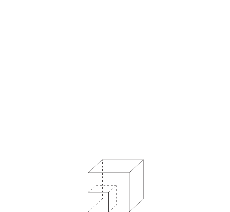
3
Random vectors in high dimensions
In this chapter we study the distributions of random vectors X = (X
1
, . . . , X
n
) ∈
R
n
where the dimension n is typically very large. Examples of high-dimensional
distributions abound in data science. For instance, computational biologists study
the expressions of n ∼ 10
4
genes in the human genome, which can be modeled as
a random vector X = (X
1
, . . . , X
n
) that encodes the gene expressions of a person
randomly drawn from a given population.
Life in high dimensions presents new challenges, which stem from the fact that
there is exponentially more room in higher dimensions than in lower dimensions.
For example, in R
n
the volume of a cube of side 2 is 2
n
times larger than the
volume of a unit cube, even though the sides of the cubes are just a factor 2
apart (see Figure 3.1). The abundance of room in higher dimensions makes many
algorithmic tasks exponentially more difficult, a phenomenon known as the “curse
of dimensionality”.
0 1 2
Figure 3.1 The abundance of room in high dimensions: the larger cube has
volume exponentially larger than the smaller cube.
Probability in high dimensions offers an array of tools to circumvent these
difficulties; some examples will be given in this chapter. We start by examining
the Euclidean norm ∥X∥
2
of a random vector X with independent coordinates,
and we show in Section 3.1 that the norm concentrates tightly about its mean.
Further basic results and examples of high-dimensional distributions (multivariate
normal, spherical, Bernoulli, frames, etc.) are covered in Section 3.2, which also
discusses principal component analysis, a powerful data exploratory procedure.
In Section 3.5 we give a probabilistic proof of the classical Grothendieck’s
inequality, and give an application to semidefinite optimization. We show that
41
42 Random vectors in high dimensions
one can sometimes relax hard optimization problems to tractable, semidefinite
programs, and use Grothendieck’s inequality to analyze the quality of such relax-
ations. In Section 3.6 we give a remarkable example of a semidefinite relaxation
of a hard optimization problem – finding the maximum cut of a given graph. We
present there the classical Goemans-Williamson randomized approximation algo-
rithm for the maximum cut problem. In Section 3.7 we give an alternative proof
of Grothendieck’s inequality (and with almost the best known constant) by in-
troducing the kernel trick, a method that has significant applications in machine
learning.
3.1 Concentration of the norm
Where in the space R
n
is a random vector X = (X
1
, . . . , X
n
) likely to be located?
Assume the coordinates X
i
are independent random variables with zero means
and unit variances. What length do we expect X to have? We have
E ∥X∥
2
2
= E
n
X
i=1
X
2
i
=
n
X
i=1
E X
2
i
= n.
So we should expect the length of X to be
∥X∥
2
≈
√
n.
We will see now that X is indeed very close to
√
n with high probability.
Theorem 3.1.1 (Concentration of the norm). Let X = (X
1
, . . . , X
n
) ∈ R
n
be a
random vector with independent, sub-gaussian coordinates X
i
that satisfy E X
2
i
=
1. Then
∥X∥
2
−
√
n
ψ
2
≤ CK
2
,
where K = max
i
∥X
i
∥
ψ
2
and C is an absolute constant.
1
Proof For simplicity, we assume that K ≥ 1. (Argue that you can make this
assumption.) We shall apply Bernstein’s deviation inequality for the normalized
sum of independent, mean zero random variables
1
n
∥X∥
2
2
− 1 =
1
n
n
X
i=1
(X
2
i
− 1).
Since the random variable X
i
is sub-gaussian, X
2
i
− 1 is sub-exponential, and
more precisely
∥X
2
i
− 1∥
ψ
1
≤ C∥X
2
i
∥
ψ
1
(by centering, see Exercise 2.7.10)
= C∥X
i
∥
2
ψ
2
(by Lemma 2.7.6)
≤ CK
2
.
1
From now on, we will always denote various positive absolute constants by C, c, C
1
, c
1
without
saying this explicitly.

3.1 Concentration of the norm 43
Applying Bernstein’s inequality (Corollary 2.8.3), we obtain for any u ≥ 0 that
P
(
1
n
∥X∥
2
2
− 1
≥ u
)
≤ 2 exp
−
cn
K
4
min(u
2
, u)
. (3.1)
(Here we used that K
4
≥ K
2
since we assumed that K ≥ 1.)
This is a good concentration inequality for ∥X∥
2
2
, from which we are going to
deduce a concentration inequality for ∥X∥
2
. To make the link, we can use the
following elementary observation that is valid for all numbers z ≥ 0:
|z − 1| ≥ δ implies |z
2
− 1| ≥ max(δ, δ
2
). (3.2)
(Check it!) We obtain for any δ ≥ 0 that
P
1
√
n
∥X∥
2
− 1
≥ δ
≤ P
(
1
n
∥X∥
2
2
− 1
≥ max(δ, δ
2
)
)
(by (3.2))
≤ 2 exp
−
cn
K
4
· δ
2
(by (3.1) for u = max(δ, δ
2
)).
Changing variables to t = δ
√
n, we obtain the desired sub-gaussian tail
P
∥X∥
2
−
√
n
≥ t
≤ 2 exp
−
ct
2
K
4
for all t ≥ 0. (3.3)
As we know from Section 2.5.2, this is equivalent to the conclusion of the theorem.
Remark 3.1.2 (Deviation). Theorem 3.1.1 states that with high probability,
X takes values very close to the sphere of radius
√
n. In particular, with high
probability (say, 0.99), X even stays within constant distance from that sphere.
Such small, constant deviations could be surprising at the first sight, so let us
explain this intuitively. The square of the norm, S
n
:
= ∥X∥
2
2
has mean n and
standard deviation O(
√
n). (Why?) Thus ∥X∥
2
=
√
S
n
ought to deviate by O(1)
around
√
n. This is because
q
n ± O(
√
n) =
√
n ± O(1);
see Figure 3.2 for an illustration.
Remark 3.1.3 (Anisotropic distributions). After we develop more tools, we will
prove a generalization of Theorem 3.1.1 for anisotropic random vectors X; see
Theorem 6.3.2.
Exercise 3.1.4 (Expectation of the norm). KKK
(a) Deduce from Theorem 3.1.1 that
√
n − CK
2
≤ E ∥X∥
2
≤
√
n + CK
2
.
(b) Can CK
2
be replaced by o(1), a quantity that vanishes as n → ∞?

44 Random vectors in high dimensions
Figure 3.2 Concentration of the norm of a random vector X in R
n
. While
∥X∥
2
2
deviates by O(
√
n) around n, ∥X∥
2
deviates by O(1) around
√
n.
Exercise 3.1.5 (Variance of the norm). KKK Deduce from Theorem 3.1.1
that
Var(∥X∥
2
) ≤ CK
4
.
Hint: Use Exercise 3.1.4.
The result of the last exercise actually holds not only for sub-gaussian distri-
butions, but for all distributions with bounded fourth moment:
Exercise 3.1.6 (Variance of the norm under finite moment assumptions). KKK
Let X = (X
1
, . . . , X
n
) ∈ R
n
be a random vector with independent coordinates
X
i
that satisfy E X
2
i
= 1 and E X
4
i
≤ K
4
. Show that
Var(∥X∥
2
) ≤ CK
4
.
Hint: First check that E(∥X∥
2
2
− n)
2
≤ K
4
n by expansion. This yields in a simple way that E(∥X∥
2
−
√
n)
2
≤ K
4
. Finally, replace
√
n by E ∥X∥
2
arguing like in Exercise 3.1.4.
Exercise 3.1.7 (Small ball probabilities). KK Let X = (X
1
, . . . , X
n
) ∈ R
n
be
a random vector with independent coordinates X
i
with continuous distributions.
Assume that the densities of X
i
are uniformly bounded by 1. Show that, for any
ε > 0, we have
P
n
∥X∥
2
≤ ε
√
n
o
≤ (Cε)
n
.
Hint: While this inequality does not follow from the result of Exercise 2.2.10 (why?), you can prove it
by a similar argument.
3.2 Covariance matrices and principal component analysis
In the last section we considered a special class of random variables, those with
independent coordinates. Before we study more general situations, let us recall
3.2 Covariance and isotropy 45
a few basic notions about high-dimensional distributions, which the reader may
have already seen in basic courses.
The concept of the mean of a random variable generalizes in a straightforward
way for a random vectors X taking values in R
n
. The notion of variance is replaced
in high dimensions by the covariance matrix of a random vector X ∈ R
n
, defined
as follows:
cov(X) = E(X − µ)(X − µ)
T
= E XX
T
− µµ
T
, where µ = E X.
Thus cov(X) is an n×n, symmetric positive semidefinite matrix. The formula for
covariance is a direct high-dimensional generalization of the definition of variance
for a random variables Z, which is
Var(Z) = E(Z − µ)
2
= E Z
2
− µ
2
, where µ = E Z.
The entries of cov(X) are the covariances of the pairs of coordinates of X =
(X
1
, . . . , X
n
):
cov(X)
ij
= E(X
i
− E X
i
)(X
j
− E X
j
).
It is sometimes useful to consider the second moment matrix of a random vector
X, defined as
Σ = Σ(X) = E XX
T
.
The second moment matrix is a higher dimensional generalization of the second
moment E Z
2
of a random variable Z. By translation (replacing X with X − µ),
we can assume in many problems that X has zero mean, and thus covariance and
second moment matrices are equal:
cov(X) = Σ(X).
This observation allows us to mostly focus on the second moment matrix Σ =
Σ(X) rather than on the covariance cov(X) in the future.
Like the covariance matrix, the second moment matrix Σ is also an n×n, sym-
metric and positive semidefinite matrix. The spectral theorem for such matrices
says that all eigenvalues s
i
of Σ are real and non-negative. Moreover, Σ can be
expressed via spectral decomposition as
Σ =
n
X
i=1
s
i
u
i
u
T
i
,
where u
i
∈ R
n
are the eigenvectors of Σ. We usually arrange the terms in this
sum so that the eigenvalues s
i
are decreasing.
3.2.1 Principal component analysis
The spectral decomposition of Σ is of utmost importance in applications where
the distribution of a random vector X in R
n
represents data, for example the
genetic data we mentioned on p. 41. The eigenvector u
1
corresponding to the
largest eigenvalue s
1
defines the first principal direction. This is the direction in

46 Random vectors in high dimensions
which the distribution is most extended, and it explains most of the variability in
the data. The next eigenvector u
2
(corresponding to the next largest eigenvalue
s
2
) defines the next principal direction; it best explains the remaining variations
in the data, and so on. This is illustrated in the Figure 3.3.
Figure 3.3 Illustration of the PCA. 200 sample points are shown from a
distribution in R
2
. The covariance matrix Σ has eigenvalues s
i
and
eigenvectors u
i
.
It often happens with real data that only a few eigenvalues s
i
are large and can
be considered as informative; the remaining eigenvalues are small and considered
as noise. In such situations, a few principal directions can explain most variability
in the data. Even though the data is presented in a high-dimensional space R
n
,
such data is essentially low dimensional. It clusters near the low-dimensional
subspace E spanned by the first few principal components.
The most basic data analysis algorithm, called the principal component analysis
(PCA), computes the first few principal components and then projects the data
in R
n
onto the subspace E spanned by them. This considerably reduces the
dimension of the data and simplifies the data analysis. For example, if E is two-
or three-dimensional, PCA allows one to visualize the data.
3.2.2 Isotropy
We might remember from a basic probability course how it is often convenient to
assume that random variables have zero means and unit variances. This is also
true in higher dimensions, where the notion of isotropy generalizes the assumption
of unit variance.
Definition 3.2.1 (Isotropic random vectors). A random vector X in R
n
is called
isotropic if
Σ(X) = E XX
T
= I
n
where I
n
denotes the identity matrix in R
n
.
Recall that any random variable X with positive variance can be reduced by
translation and dilation to the standard score – a random variable Z with zero
mean and unit variance, namely
Z =
X − µ
p
Var(X)
.

3.2 Covariance and isotropy 47
The following exercise gives a high-dimensional version of standard score.
Exercise 3.2.2 (Reduction to isotropy). K
(a) Let Z be a mean zero, isotropic random vector in R
n
. Let µ ∈ R
n
be a
fixed vector and Σ be a fixed n×n symmetric positive semidefinite matrix.
Check that the random vector
X
:
= µ + Σ
1/2
Z
has mean µ and covariance matrix cov(X) = Σ.
(b) Let X be a random vector with mean µ and invertible covariance matrix
Σ = cov(X). Check that the random vector
Z
:
= Σ
−1/2
(X − µ)
is an isotropic, mean zero random vector.
This observation will allow us in many future results about random vectors to
assume without loss of generality that they have zero means and are isotropic.
3.2.3 Properties of isotropic distributions
Lemma 3.2.3 (Characterization of isotropy). A random vector X in R
n
is
isotropic if and only if
E ⟨X, x⟩
2
= ∥x∥
2
2
for all x ∈ R
n
.
Proof Recall that two symmetric n ×n matrices A and B are equal if and only
if x
T
Ax = x
T
Bx for all x ∈ R
n
. (Check this!) Thus X is isotropic if and only if
x
T
E XX
T
x = x
T
I
n
x for all x ∈ R
n
.
The left side of this identity equals E ⟨X, x⟩
2
and the right side is ∥x∥
2
2
. This
completes the proof.
If x is a unit vector in Lemma 3.2.3, we can view ⟨X, x⟩ as a one-dimensional
marginal of the distribution of X, obtained by projecting X onto the direction
of x. Then a mean-zero random vector X is isotropic if and only if all one-
dimensional marginals of X have unit variance. Informally, this means that an
isotropic distribution is extended evenly in all directions.
Lemma 3.2.4. Let X be an isotropic random vector in R
n
. Then
E ∥X∥
2
2
= n.
Moreover, if X and Y are two independent isotropic random vectors in R
n
, then
E ⟨X, Y ⟩
2
= n.

48 Random vectors in high dimensions
Proof To prove the first part, we have
E ∥X∥
2
2
= E X
T
X = E tr(X
T
X) (viewing X
T
X as a 1 × 1 matrix)
= E tr(XX
T
) (by the cyclic property of trace)
= tr(E XX
T
) (by linearity)
= tr(I
n
) (by isotropy)
= n.
To prove the second part, we use a conditioning argument. Fix a realization of Y
and take the conditional expectation (with respect to X) which we denote E
X
.
The law of total expectation says that
E ⟨X, Y ⟩
2
= E
Y
E
X
h
⟨X, Y ⟩
2
|Y
i
,
where by E
Y
we of course denote the expectation with respect to Y . To compute
the inner expectation, we apply Lemma 3.2.3 with x = Y and conclude that the
inner expectation equals ∥Y ∥
2
2
. Thus
E ⟨X, Y ⟩
2
= E
Y
∥Y ∥
2
2
= n (by the first part of lemma).
The proof is complete.
Remark 3.2.5 (Almost orthogonality of independent vectors). Let us normalize
the random vectors X and Y in Lemma 3.2.4, setting
X
:
=
X
∥X∥
2
and Y
:
=
Y
∥Y ∥
2
.
Lemma 3.2.4 is basically telling us that
2
∥X∥
2
≍
√
n, ∥Y ∥
2
≍
√
n and ⟨X, Y ⟩ ≍
√
n with high probability, which implies that
D
X, Y
E
≍
1
√
n
Thus, in high-dimensional spaces independent and isotropic random vectors tend
to be almost orthogonal, see Figure 3.4.
X
Y
Y
X
π/4
π/2
Figure 3.4 Independent isotropic random vectors tend to be almost
orthogonal in high dimensions but not in low dimensions. On the plane, the
average angle is π/4, while in high dimensions it is close to π/2.
2
This argument is not entirely rigorous, since Lemma 3.2.4 is about expectation and not high
probability. To make it more rigorous, one can use Theorem 3.1.1 about concentration of the norm.

3.3 Examples of high-dimensional distributions 49
This may sound surprising since this is not the case in low dimensions. For
example, the angle between two random independent and uniformly distributed
directions on the plane has mean π/4. (Check!) But in higher dimensions, there
is much more room as we mentioned in the beginning of this chapter. This is
an intuitive reason why random directions in high-dimensional spaces tend to be
very far from each other, i.e. almost orthogonal.
Exercise 3.2.6 (Distance between independent isotropic vectors). K Let X
and Y be independent, mean zero, isotropic random vectors in R
n
. Check that
E ∥X − Y ∥
2
2
= 2n.
3.3 Examples of high-dimensional distributions
In this section we give several basic examples of isotropic high-dimensional dis-
tributions.
3.3.1 Spherical and Bernoulli distributions
The coordinates of an isotropic random vector are always uncorrelated (why?),
but they are not necessarily independent. An example of this situation is the
spherical distribution, where a random vector X is uniformly distributed
3
on the
Euclidean sphere in R
n
with center at the origin and radius
√
n:
X ∼ Unif
√
n S
n−1
.
Exercise 3.3.1. K Show that the spherically distributed random vector X is
isotropic. Argue that the coordinates of X are not independent.
A good example of a discrete isotropic distribution in R
n
is the symmetric
Bernoulli distribution. We say that a random vector X = (X
1
, . . . , X
n
) is sym-
metric Bernoulli if the coordinates X
i
are independent, symmetric Bernoulli ran-
dom variables. Equivalently, we may say that X is uniformly distributed on the
unit discrete cube in R
n
:
X ∼ Unif
{−1, 1}
n
.
The symmetric Bernoulli distribution is isotropic. (Check!)
More generally, we may consider any random vector X = (X
1
, . . . , X
n
) whose
coordinates X
i
are independent random variables with zero mean and unit vari-
ance. Then X is an isotropic vector in R
n
. (Why?)
3
More rigorously, we say that X is uniformly distributed on
√
n S
n−1
if, for every (Borel) subset
E ⊂ S
n−1
, the probability P
n
X ∈ E
o
equals the ratio of the (n − 1)-dimensional areas of E and
S
n−1
.

50 Random vectors in high dimensions
3.3.2 Multivariate normal
One of the most important high-dimensional distributions is Gaussian, or multi-
variate normal. From a basic probability course we know that a random vector
g = (g
1
, . . . , g
n
) has the standard normal distribution in R
n
, denoted
g ∼ N(0, I
n
),
if the coordinates g
i
are independent standard normal random variables N (0, 1).
The density of Z is then the product of the n standard normal densities (1.6),
which is
f(x) =
n
Y
i=1
1
√
2π
e
−x
2
i
/2
=
1
(2π)
n/2
e
−∥x∥
2
2
/2
, x ∈ R
n
. (3.4)
The standard normal distribution is isotropic. (Why?)
Note that the standard normal density (3.4) is rotation invariant, since f(x)
depends only on the length but not the direction of x. We can equivalently express
this observation as follows:
Proposition 3.3.2 (Rotation invariance). Consider a random vector g ∼ N(0, I
n
)
and a fixed orthogonal matrix U. Then
Ug ∼ N(0, I
n
).
Exercise 3.3.3 (Rotation invariance). KK Deduce the following properties
from the rotation invariance of the normal distribution.
(a) Consider a random vector g ∼ N (0, I
n
) and a fixed vector u ∈ R
n
. Then
⟨g, u⟩ ∼ N (0, ∥u∥
2
2
).
(b) Consider independent random variables X
i
∼ N(0, σ
2
i
). Then
n
X
i=1
X
i
∼ N(0, σ
2
) where σ
2
=
n
X
i=1
σ
2
i
.
(c) Let G be an m × n Gaussian random matrix, i.e. the entries of G are
independent N (0, 1) random variables. Let u ∈ R
n
be a fixed unit vector.
Then
Gu ∼ N(0, I
m
).
Let us also recall the notion of the general normal distribution N (µ, Σ). Con-
sider a vector µ ∈ R
n
and an invertible n × n positive semidefinite matrix Σ.
According to Exercise 3.2.2, the random vector X
:
= µ + Σ
1/2
Z has mean µ and
covariance matrix Σ(X) = Σ. Such X is said to have a general normal distribution
in R
n
, denoted
X ∼ N(µ, Σ).
Summarizing, we have X ∼ N (µ, Σ) if and only if
Z
:
= Σ
−1/2
(X − µ) ∼ N (0, I
n
).

3.3 Examples of high-dimensional distributions 51
The density of X ∼ N (µ, Σ) can be computed by the change of variables formula,
and it equals
f
X
(x) =
1
(2π)
n/2
det(Σ)
1/2
e
−(x−µ)
T
Σ
−1
(x−µ)/2
, x ∈ R
n
. (3.5)
Figure 3.5 shows examples of two densities of multivariate normal distributions.
An important observation is that the coordinates of a random vector X ∼
N(µ, Σ) are independent if and only if they are uncorrelated. (In this case Σ = I
n
.)
Exercise 3.3.4 (Characterization of normal distribution). KKK Let X be a
random vector in R
n
. Show that X has a multivariate normal distribution if and
only if every one-dimensional marginal ⟨X, θ⟩, θ ∈ R
n
, has a (univariate) normal
distribution.
Hint: Utilize a version of Cram´er-Wold’s theorem, which states that the totality of the distributions of
one-dimensional marginals determine the distribution in R
n
uniquely. More precisely, if X and Y are
random vectors in R
n
such that ⟨X, θ⟩ and ⟨Y, θ⟩ have the same distribution for each θ ∈ R
n
, then X
and Y have the same distribution.
Figure 3.5 The densities of the isotropic distribution N (0, I
2
) and a
non-isotropic distribution N(0, Σ).
Exercise 3.3.5. K Let X ∼ N(0, I
n
).
(a) Show that, for any fixed vectors u, v ∈ R
n
, we have
E ⟨X, u⟩⟨X, v⟩ = ⟨u, v⟩. (3.6)
(b) Given a vector u ∈ R
n
, consider the random variable X
u
:
= ⟨X, u⟩. From
Exercise 3.3.3 we know that X
u
∼ N(0, ∥u∥
2
2
). Check that
∥X
u
− X
v
∥
L
2
= ∥u − v∥
2
for any fixed vectors u, v ∈ R
n
. (Here ∥·∥
L
2
denotes the norm in the Hilbert
space L
2
of random variables, which we introduced in (1.1).)
Exercise 3.3.6. K Let G be an m×n Gaussian random matrix, i.e. the entries
of G are independent N(0, 1) random variables. Let u, v ∈ R
n
be unit orthogonal
vectors. Prove that Gu and Gv are independent N(0, I
m
) random vectors.
Hint: Reduce the problem to the case where u and v are collinear with canonical basis vectors of R
n
.

52 Random vectors in high dimensions
3.3.3 Similarity of normal and spherical distributions
Contradicting our low dimensional intuition, the standard normal distribution
N(0, I
n
) in high dimensions is not concentrated close to the origin, where the
density is maximal. Instead, it is concentrated in a thin spherical shell around the
sphere of radius
√
n, a shell of width O(1). Indeed, the concentration inequality
(3.3) for the norm of g ∼ N(0, I
n
) states that
P
∥g∥
2
−
√
n
≥ t
≤ 2 exp(−ct
2
) for all t ≥ 0. (3.7)
This observation suggests that the normal distribution should be quite similar
to the uniform distribution on the sphere. Let us clarify the relation.
Exercise 3.3.7 (Normal and spherical distributions). K Let us represent g ∼
N(0, I
n
) in polar form as
g = rθ
where r = ∥g∥
2
is the length and θ = g/∥g∥
2
is the direction of g. Prove the
following:
(a) The length r and direction θ are independent random variables.
(b) The direction θ is uniformly distributed on the unit sphere S
n−1
.
Concentration inequality (3.7) says that r = ∥g∥
2
≈
√
n with high probability,
so
g ≈
√
n θ ∼ Unif
√
nS
n−1
.
In other words, the standard normal distribution in high dimensions is close to
the uniform distribution on the sphere of radius
√
n, i.e.
N(0, I
n
) ≈ Unif
√
nS
n−1
. (3.8)
Figure 3.6 illustrates this fact that goes against our intuition that has been trained
in low dimensions.
3.3.4 Frames
For an example of an extremely discrete distribution, consider a coordinate ran-
dom vector X uniformly distributed in the set {
√
n e
i
}
n
i=1
where {e
i
}
n
i=1
is the
canonical basis of R
n
:
X ∼ Unif
n
√
n e
i
:
i = 1, . . . , n
o
.
Then X is an isotropic random vector in R
n
. (Check!)
Of all high-dimensional distributions, Gaussian is often the most convenient to
prove results for, so we may think of it as “the best” distribution. The coordinate
distribution, the most discrete of all distributions, is “the worst”.
A general class of discrete, isotropic distributions arises in the area of signal
processing under the name of frames.
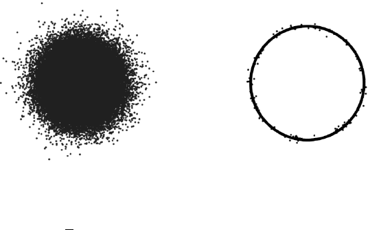
3.3 Examples of high-dimensional distributions 53
Figure 3.6 A Gaussian point cloud in two dimensions (left) and its
intuitive visualization in high dimensions (right). In high dimensions, the
standard normal distribution is very close to the uniform distribution on the
sphere of radius
√
n.
Definition 3.3.8. A frame is a set of vectors {u
i
}
N
i=1
in R
n
which obeys an
approximate Parseval’s identity, i.e. there exist numbers A, B > 0 called frame
bounds such that
A∥x∥
2
2
≤
N
X
i=1
⟨u
i
, x⟩
2
≤ B∥x∥
2
2
for all x ∈ R
n
.
If A = B the set {u
i
}
N
i=1
is called a tight frame.
Exercise 3.3.9. KK Show that {u
i
}
N
i=1
is a tight frame in R
n
with bound A if
and only if
N
X
i=1
u
i
u
T
i
= AI
n
. (3.9)
Hint: Proceed similarly to the proof of Lemma 3.2.3.
Multiplying both sides of (3.9) by a vector x, we see that
N
X
i=1
⟨u
i
, x⟩u
i
= Ax for any x ∈ R
n
. (3.10)
This is a frame expansion of a vector x, and it should look familiar. Indeed, if
{u
i
} is an orthonormal basis, then (3.10) is just a classical basis expansion of x,
and it holds with A = 1.
We can think of tight frames as generalizations of orthogonal bases without the
linear independence requirement. Any orthonormal basis in R
n
is clearly a tight
frame. But so is the “Mercedez-Benz frame”, a set of three equidistant points on
a circle in R
2
shown on Figure 3.7.
Now we are ready to connect the concept of frames to probability. We show
that tight frames correspond to isotropic distributions, and vice versa.
Lemma 3.3.10 (Tight frames and isotropic distributions). (a) Consider a tight

54 Random vectors in high dimensions
Figure 3.7 the Mercedes-Benz frame. A set of equidistant points on the
circle form a tight frame in R
2
.
frame {u
i
}
N
i=1
in R
n
with frame bounds A = B. Let X be a random vector
that is uniformly distributed in the set of frame elements, i.e.
X ∼ Unif {u
i
:
i = 1, . . . , N}.
Then (N/A)
1/2
X is an isotropic random vector in R
n
.
(b) Consider an isotropic random vector X in R
n
that takes a finite set of
values x
i
with probabilities p
i
each, i = 1, . . . , N. Then the vectors
u
i
:
=
√
p
i
x
i
, i = 1, . . . , N,
form a tight frame in R
n
with bounds A = B = 1.
Proof 1. Without loss of generality, we can assume that A = N. (Why?) The
assumptions and (3.9) imply that
N
X
i=1
u
i
u
T
i
= NI
n
.
Dividing both sides by N and interpreting
1
N
P
N
i=1
as an expectation, we conclude
that X is isotropic.
2. Isotropy of X means that
E XX
T
=
N
X
i=1
p
i
x
i
x
T
i
= I
n
.
Denoting u
i
:
=
√
p
i
x
i
, we obtain (3.9) with A = 1.
3.3.5 Isotropic convex sets
Our last example of a high-dimensional distribution comes from convex geometry.
Consider a bounded convex set K in R
n
with non-empty interior; such sets are
called convex bodies. Let X be a random vector uniformly distributed in K,
according to the probability measure given by normalized volume in K:
X ∼ Unif(K).

3.4 Sub-gaussian distributions in higher dimensions 55
Assume that E X = 0 (translate K appropriately to achieve this) and denote
the covariance matrix of X by Σ. Then by Exercise 3.2.2, the random vector
Z
:
= Σ
−1/2
X is isotropic. Note that Z is uniformly distributed in the linearly
transformed copy of K:
Z ∼ Unif(Σ
−1/2
K).
(Why?) Summarizing, we found a linear transformation T
:
= Σ
−1/2
which makes
the uniform distribution on T K isotropic. The body T K is sometimes called
isotropic itself.
In algorithmic convex geometry, one can think of the isotropic convex body TK
as a well conditioned version of K, with T playing the role of a pre-conditioner,
see Figure 3.8. Algorithms related to convex bodies K (such as computing the
volume of K) tend to work better for well-conditioned bodies K.
Figure 3.8 A convex body K on the left is transformed into an isotropic
convex body T K on the right. The pre-conditioner T is computed from the
covariance matrix Σ of K as T = Σ
−1/2
.
3.4 Sub-gaussian distributions in higher dimensions
The concept of sub-gaussian distributions, which we introduced in Section 2.5,
can be extended to higher dimensions. To see how, recall from Exercise 3.3.4
that the multivariate normal distribution can be characterized through its one-
dimensional marginals, or projections onto lines: a random vector X has a normal
distribution in R
n
if and only if the one-dimensional marginals ⟨X, x⟩ are normal
for all x ∈ R
n
. Guided by this characterization, it is natural to define multivariate
sub-gaussian distributions as follows.
Definition 3.4.1 (Sub-gaussian random vectors). A random vector X in R
n
is called sub-gaussian if the one-dimensional marginals ⟨X, x⟩ are sub-gaussian
random variables for all x ∈ R
n
. The sub-gaussian norm of X is defined as
∥X∥
ψ
2
= sup
x∈S
n−1
∥⟨X, x⟩∥
ψ
2
.
A good example of a sub-gaussian random vector is a random vector with
independent, sub-gaussian coordinates:
Lemma 3.4.2 (Sub-gaussian distributions with independent coordinates). Let

56 Random vectors in high dimensions
X = (X
1
, . . . , X
n
) ∈ R
n
be a random vector with independent, mean zero, sub-
gaussian coordinates X
i
. Then X is a sub-gaussian random vector, and
∥X∥
ψ
2
≤ C max
i≤n
∥X
i
∥
ψ
2
.
Proof This is an easy consequence of the fact that a sum of independent sub-
gaussian random variables is sub-gaussian, which we proved in Proposition 2.6.1.
Indeed, for a fixed unit vector x = (x
1
, . . . , x
n
) ∈ S
n−1
we have
∥⟨X, x⟩∥
2
ψ
2
=
n
X
i=1
x
i
X
i
2
ψ
2
≤ C
n
X
i=1
x
2
i
∥X
i
∥
2
ψ
2
(by Proposition 2.6.1)
≤ C max
i≤n
∥X
i
∥
2
ψ
2
(using that
n
X
i=1
x
2
i
= 1).
This completes the proof.
Exercise 3.4.3. KK This exercise clarifies the role of independence of coordi-
nates in Lemma 3.4.2.
1. Let X = (X
1
, . . . , X
n
) ∈ R
n
be a random vector with sub-gaussian coordi-
nates X
i
. Show that X is a sub-gaussian random vector.
2. Nevertheless, find an example of a random vector X with
∥X∥
ψ
2
≫ max
i≤n
∥X
i
∥
ψ
2
.
Many important high-dimensional distributions are sub-gaussian, but some are
not. We now explore some basic distributions.
3.4.1 Gaussian and Bernoulli distributions
As we already noted, multivariate normal distribution N(µ, Σ) is sub-gaussian.
Moreover, the standard normal random vector X ∼ N(0, I
n
) has sub-gaussian
norm of order O(1):
∥X∥
ψ
2
≤ C.
(Indeed, all one-dimensional marginals of X are N(0, 1).)
Next, consider the multivariate symmetric Bernoulli distribution that we intro-
duced in Section 3.3.1. A random vector X with this distribution has independent,
symmetric Bernoulli coordinates, so Lemma 3.4.2 yields that
∥X∥
ψ
2
≤ C.
3.4.2 Discrete distributions
Let us now pass to discrete distributions. The extreme example we considered
in Section 3.3.4 is the coordinate distribution. Recall that random vector X with
coordinate distribution is uniformly distributed in the set {
√
ne
i
:
i = 1, . . . , n},
where e
i
denotes the the n-element set of the canonical basis vectors in R
n
.

3.4 Sub-gaussian distributions in higher dimensions 57
Is X sub-gaussian? Formally, yes. In fact, every distribution supported in a fi-
nite set is sub-gaussian. (Why?) But, unlike Gaussian and Bernoulli distributions,
the coordinate distribution has a very large sub-gaussian norm.
Exercise 3.4.4. K Show that
∥X∥
ψ
2
≍
r
n
log n
.
Such large norm makes it useless to think of X as a sub-gaussian random
vector.
More generally, discrete distributions do not make nice sub-gaussian distribu-
tions, unless they are supported on exponentially large sets:
Exercise 3.4.5. KKKK Let X be an isotropic random vector supported in a
finite set T ⊂ R
n
. Show that in order for X to be sub-gaussian with ∥X∥
ψ
2
=
O(1), the cardinality of the set must be exponentially large in n:
|T | ≥ e
cn
.
In particular, this observation rules out frames (see Section 3.3.4) as good sub-
gaussian distributions unless they have exponentially many terms (in which case
they are mostly useless in practice).
3.4.3 Uniform distribution on the sphere
In all previous examples, good sub-gaussian random vectors had independent
coordinates. This is not necessary. A good example is the uniform distribution
on the sphere of radius
√
n, which we discussed in Section 3.3.1. We will show
that it is sub-gaussian by reducing it to the Gaussian distribution N (0, I
n
).
Theorem 3.4.6 (Uniform distribution on the sphere is sub-gaussian). Let X be
a random vector uniformly distributed on the Euclidean sphere in R
n
with center
at the origin and radius
√
n:
X ∼ Unif
√
n S
n−1
.
Then X is sub-gaussian, and
∥X∥
ψ
2
≤ C.
Proof Consider a standard normal random vector g ∼ N(0, I
n
). As we noted in
Exercise 3.3.7, the direction g/∥g∥
2
is uniformly distributed on the unit sphere
S
n−1
. Thus, by rescaling we can represent a random vector X ∼ Unif
√
n S
n−1
as
X =
√
n
g
∥g∥
2
.
We need to show that all one-dimensional marginals ⟨X, x⟩ are sub-gaussian.

58 Random vectors in high dimensions
By rotation invariance, we may assume that x = (1, 0, . . . , 0), in which case
⟨X, x⟩ = X
1
, the first coordinate of X. We want to bound the tail probability
p(t)
:
= P
|X
1
| ≥ t
= P
(
|g
1
|
∥g∥
2
≥
t
√
n
)
.
The concentration of norm (Theorem 3.1.1) implies that
∥g∥
2
≈
√
n with high probability.
This reduces the problem to bounding P
|g
1
| ≥ t
, but as we know from (2.3),
this tail is sub-gaussian.
Let us do this argument more carefully. Theorem 3.1.1 implies that
∥g∥
2
−
√
n
ψ
2
≤ C.
Thus the event
E
:
=
(
∥g∥
2
≥
√
n
2
)
is likely: by (2.14) its complement E
c
has probability
P(E
c
) ≤ 2 exp(−cn). (3.11)
Then the tail probability can be bounded as follows:
p(t) ≤ P
(
|g
1
|
∥g∥
2
≥
t
√
n
and E
)
+ P(E
c
)
≤ P
|g
1
| ≥
t
2
and E
+ 2 exp(−cn) (by definition of E and (3.11))
≤ 2 exp(−t
2
/8) + 2 exp(−cn) (drop E and use (2.3)).
Consider two cases. If t ≤
√
n then 2 exp(−cn) ≤ 2 exp(−ct
2
/8), and we con-
clude that
p(t) ≤ 4 exp(−c
′
t
2
)
as desired. In the opposite case where t >
√
n, the tail probability p(t) =
P
|X
1
| ≥ t
trivially equals zero, since we always have |X
1
| ≤ ∥X∥
2
=
√
n.
This completes the proof by the characterization of sub-gaussian distributions
(recall Proposition 2.5.2 and Remark 2.5.3).
Exercise 3.4.7 (Uniform distribution on the Euclidean ball). KK Extend The-
orem 3.4.6 for the uniform distribution on the Euclidean ball B(0,
√
n) in R
n
centered at the origin and with radius
√
n. Namely, show that a random vector
X ∼ Unif
B(0,
√
n)
is sub-gaussian, and
∥X∥
ψ
2
≤ C.

3.4 Sub-gaussian distributions in higher dimensions 59
Remark 3.4.8 (Projective limit theorem). Theorem 3.4.6 should be compared to
the so-called projective central limit theorem. It states that the marginals of the
uniform distribution on the sphere become asymptotically normal as n increases,
see Figure 3.9. Precisely, if X ∼ Unif
√
n S
n−1
then for any fixed unit vector x
we have
⟨X, x⟩ → N(0, 1) in distribution as n → ∞.
Thus we can view Theorem 3.4.6 as a concentration version of the Projective
Limit Theorem, in the same sense as Hoeffding’s inequality in Section 2.2 is a
concentration version of the classical central limit theorem.
Figure 3.9 The projective central limit theorem: the projection of the
uniform distribution on the sphere of radius
√
n onto a line converges to the
normal distribution N(0, 1) as n → ∞.
3.4.4 Uniform distribution on convex sets
To conclude this section, let us return to the class of uniform distributions on
convex sets which we discussed in Section 3.3.5. Let K be a convex body and
X ∼ Unif(K)
be an isotropic random vector. Is X always sub-gaussian?
For some bodies K, this is the case. Examples include the Euclidean ball of ra-
dius
√
n (by Exercise 3.4.7) and the unit cube [−1, 1]
n
(according to Lemma 3.4.2).
For some other bodies, this is not true:
Exercise 3.4.9. KKK Consider a ball of the ℓ
1
norm in R
n
:
K
:
=
x ∈ R
n
:
∥x∥
1
≤ r
.
(a) Show that the uniform distribution on K is isotropic for some r ≍ n.
(b) Show that the subgaussian norm of this distribution is not bounded by an
absolute constant as the dimension n grows.
Nevertheless, it is possible to prove a weaker result for a general isotropic convex
body K. The random vector X ∼ Unif(K) has all sub-exponential marginals, and
∥⟨X, x⟩∥
ψ
1
≤ C
60 Random vectors in high dimensions
for all unit vectors x. This result follows from C. Borell’s lemma, which itself is
a consequence of Brunn-Minkowski inequality; see [81, Section 2.2.b
3
].
Exercise 3.4.10. KK Show that the concentration inequality in Theorem 3.1.1
may not hold for a general isotropic sub-gaussian random vector X. Thus, inde-
pendence of the coordinates of X is an essential requirement in that result.
3.5 Application: Grothendieck’s inequality and semidefinite
programming
In this and the next section, we use high-dimensional Gaussian distributions to
pursue some problems that have seemingly nothing to do with probability. Here
we give a probabilistic proof of Grothendieck’s inequality, a remarkable result
which we will use later in the analysis of some computationally hard problems.
Theorem 3.5.1 (Grothendieck’s inequality). Consider an m ×n matrix (a
ij
) of
real numbers. Assume that, for any numbers x
i
, y
j
∈ {−1, 1}, we have
X
i,j
a
ij
x
i
y
j
≤ 1.
Then, for any Hilbert space H and any vectors u
i
, v
j
∈ H satisfying ∥u
i
∥ =
∥v
j
∥ = 1, we have
X
i,j
a
ij
u
i
, v
j
≤ K,
where K ≤ 1.783 is an absolute constant.
There is apparently nothing random in the statement of this theorem, but
our proof of this result will be probabilistic. We will actually give two proofs
of Grothendieck’s inequality. The one given in this section will yield a much
worse bound on the constant K, namely K ≤ 288. In Section 3.7, we present an
alternative argument that yields the bound K ≤ 1.783 as stated in Theorem 3.5.1.
Before we pass to the argument, let us make one simple observation.
Exercise 3.5.2. K
(a) Check that the assumption of Grothendieck’s inequality can be equivalently
stated as follows:
X
i,j
a
ij
x
i
y
j
≤ max
i
|x
i
| · max
j
|y
j
|. (3.12)
for any real numbers x
i
and y
j
.
(b) Show that the conclusion of Grothendieck’s inequality can be equivalently
stated as follows:
X
i,j
a
ij
u
i
, v
j
≤ K max
i
∥u
i
∥ · max
j
∥v
j
∥ (3.13)

3.5 Application: Grothendieck’s inequality and semidefinite programming 61
for any Hilbert space H and any vectors u
i
, v
j
∈ H.
Proof of Theorem 3.5.1 with K ≤ 288. Step 1: Reductions. Note that Gro-
thendieck’s inequality becomes trivial if we allow the value of K depend on the
matrix A = (a
ij
). (For example, K =
P
ij
|a
ij
| would work – check!) Let us choose
K = K(A) to be the smallest number that makes the conclusion (3.13) valid for
a given matrix A and any Hilbert space H and any vectors u
i
, v
j
∈ H. Our goal
is to show that K does not depend on the matrix A or the dimensions m and n.
Without loss of generality,
4
we may do this for a specific Hilbert space H,
namely for R
N
equipped with the Euclidean norm ∥·∥
2
. Let us fix vectors u
i
, v
j
∈
R
N
which realize the smallest K, that is
X
i,j
a
ij
u
i
, v
j
= K, ∥u
i
∥
2
= ∥v
j
∥
2
= 1.
Step 2: Introducing randomness. The main idea of the proof is to realize
the vectors u
i
, v
j
via Gaussian random variables
U
i
:
= ⟨g, u
i
⟩ and V
j
:
=
g, v
j
, where g ∼ N(0, I
N
).
As we noted in Exercise 3.3.5, U
i
and V
j
are standard normal random variables
whose correlations follow exactly the inner products of the vectors u
i
and v
j
:
E U
i
V
j
=
u
i
, v
j
.
Thus
K =
X
i,j
a
ij
u
i
, v
j
= E
X
i,j
a
ij
U
i
V
j
. (3.14)
Assume for a moment that the random variables U
i
and V
j
were bounded almost
surely by some constant – say, by R. Then the assumption (3.12) of Grothendieck’s
inequality (after rescaling) would yield
P
i,j
a
ij
U
i
V
j
≤ R
2
almost surely, and
(3.14) would then give K ≤ R
2
.
Step 3: Truncation. Of course, this reasoning is flawed: the random variables
U
i
, V
j
∼ N(0, 1) are not bounded almost surely. To fix this argument, we can
utilize a useful truncation trick. Let us fix some level R ≥ 1 and decompose the
random variables as follows:
U
i
= U
−
i
+ U
+
i
where U
−
i
= U
i
1
{|U
i
|≤R}
and U
+
i
= U
i
1
{|U
i
|>R}
.
We similarly decompose V
j
= V
−
j
+ V
+
j
. Now U
−
i
and V
−
j
are bounded by R
almost surely as we desired. The remainder terms U
+
i
and V
+
j
are small in the
L
2
norm: indeed, the bound in Exercise 2.1.4 gives
∥U
+
i
∥
2
L
2
≤ 2
R +
1
R
1
√
2π
e
−R
2
/2
<
4
R
2
, (3.15)
4
To see this, we can first trivially replace H with the subspace of H spanned by the vectors u
i
and v
j
(and with the norm inherited from H). This subspace has dimension at most N
:
= m + n. Next, we
recall the basic fact that all N-dimensional Hilbert spaces are isometric with each other, and in
particular they are isometric to R
N
with the norm ∥ · ∥
2
. The isometry can be constructed by
identifying orthogonal bases of those spaces.

62 Random vectors in high dimensions
and similarly for V
+
j
.
Step 4: Breaking up the sum. The sum in (3.14) becomes
K = E
X
i,j
a
ij
(U
−
i
+ U
+
i
)(V
−
j
+ V
+
j
).
When we expand the product in each term we obtain four sums, which we proceed
to bound individually. The first sum,
S
1
:
= E
X
i,j
a
ij
U
−
i
V
−
j
,
is the best of all. By construction, the random variables U
−
i
and V
−
j
are bounded
almost surely by R. Thus, just like we explained above, we can use the assumption
(3.12) of Grothendieck’s inequality to get S
1
≤ R
2
.
We are not able to use the same reasoning for the second sum,
S
2
:
= E
X
i,j
a
ij
U
+
i
V
−
j
,
since the random variable U
+
i
is unbounded. Instead, we will view the random
variables U
+
i
and V
−
j
as elements of the Hilbert space L
2
with the inner product
⟨X, Y ⟩
L
2
= E XY . The second sum becomes
S
2
=
X
i,j
a
ij
D
U
+
i
, V
−
j
E
L
2
. (3.16)
Recall from (3.15) that ∥U
+
i
∥
L
2
< 2/R and ∥V
−
j
∥
L
2
≤ ∥V
j
∥
L
2
= 1 by construction.
Then, applying the conclusion (3.13) of Grothendieck’s inequality for the Hilbert
space H = L
2
, we find that
5
S
2
≤ K ·
2
R
.
The third and fourth sums, S
3
:
= E
P
i,j
a
ij
U
−
i
V
+
j
and S
4
:
= E
P
i,j
a
ij
U
+
i
V
+
j
,
can be both bounded just like S
2
. (Check!)
Step 5: Putting everything together. Putting the four sums together, we
conclude from (3.14) that
K ≤ R
2
+
6K
R
.
Choosing R = 12 (for example) and solve the resulting inequality, we obtain
K ≤ 288. The theorem is proved.
Exercise 3.5.3 (Symmetric matrices, x
i
= y
i
). KKK Deduce the following
version of Grothendieck’s inequality for symmetric n ×n matrices A = (a
ij
) with
5
It might seem weird that we are able to apply the inequality that we are trying to prove.
Remember, however, that we chose K in the beginning of the proof as the best number that makes
Grothendieck’s inequality valid. This is the K we are using here.
3.5 Application: Grothendieck’s inequality and semidefinite programming 63
real entries. Suppose that A is either positive semidefinite or has zero diagonal.
Assume that, for any numbers x
i
∈ {−1, 1}, we have
X
i,j
a
ij
x
i
x
j
≤ 1.
Then, for any Hilbert space H and any vectors u
i
, v
j
∈ H satisfying ∥u
i
∥ =
∥v
j
∥ = 1, we have
X
i,j
a
ij
u
i
, v
j
≤ 2K, (3.17)
where K is the absolute constant from Grothendieck’s inequality.
Hint: Check and use the polarization identity ⟨Ax, y⟩ = ⟨Au, u⟩ − ⟨Av, v⟩ where u = (x + y)/2 and
v = (x − y)/2.
3.5.1 Semidefinite programming
One application area where Grothendieck’s inequality can be particularly helpful
is the analysis of certain computationally hard problems. A powerful approach to
such problems is to try and relax them to computationally simpler and more
tractable problems. This is often done using semidefinite programming, with
Grothendieck’s inequality guaranteeing the quality of such relaxations.
Definition 3.5.4. A semidefinite program is an optimization problem of the
following type:
maximize ⟨A, X⟩
:
X ⪰ 0, ⟨B
i
, X⟩ = b
i
for i = 1, . . . , m. (3.18)
Here A and B
i
are given n×n matrices and b
i
are given real numbers. The running
“variable” X is an n ×n symmetric positive semidefinite matrix, indicated by the
notation X ⪰ 0. The inner product
⟨A, X⟩ = tr(A
T
X) =
n
X
i,j=1
A
ij
X
ij
(3.19)
is the canonical inner product on the space of n × n matrices.
Note in passing that if we minimize instead of maximize in (3.18), we still get
a semidefinite program. (To see this, replace A with −A.)
Every semidefinite program is a convex program, which maximizes a linear
function ⟨A, X⟩ over a convex set of matrices. Indeed, the set of positive semidef-
inite matrices is convex (why?), and so is its intersection with the linear subspace
defined by the constraints ⟨B
i
, X⟩ = b
i
.
This is good news since convex programs are generally algorithmically tractable.
There is a variety of computationally efficient solvers available for general convex
programs, and for semidefinite programs (3.18) in particular, for example interior
point methods.

64 Random vectors in high dimensions
Semidefinite relaxations
Semidefinite programs can be designed to provide computationally efficient re-
laxations of computationally hard problems, such as this one:
maximize
n
X
i,j=1
A
ij
x
i
x
j
:
x
i
= ±1 for i = 1, . . . , n (3.20)
where A is a given n × n symmetric matrix. This is an integer optimization
problem. The feasible set consists of 2
n
vectors x = (x
i
) ∈ {−1, 1}
n
, so finding the
maximum by exhaustive search would take exponential time. Is there a smarter
way to solve the problem? This is not likely: the problem (3.20) is known to be
computationally hard in general (NP-hard).
Nonetheless, we can “relax” the problem (3.20) to a semidefinite program that
can compute the maximum approximately, up to a constant factor. To formulate
such a relaxation, let us replace in (3.20) the numbers x
i
= ±1 by their higher-
dimensional analogs – unit vectors X
i
in R
n
. Thus we consider the following
optimization problem:
maximize
n
X
i,j=1
A
ij
X
i
, X
j
:
∥X
i
∥
2
= 1 for i = 1, . . . , n. (3.21)
Exercise 3.5.5. KK Show that the optimization (3.21) is equivalent to the
following semidefinite program:
maximize ⟨A, X⟩
:
X ⪰ 0, X
ii
= 1 for i = 1, . . . , n. (3.22)
Hint: Consider the Gram matrix of the vectors X
i
, which is the n ×n matrix with entries
X
i
, X
j
. Do
not forget to describe how to translate a solution of (3.22) into a solution of (3.21).
The guarantee of relaxation
We now see how Grothendieck’s inequality guarantees the accuracy of semidefinite
relaxations: the semidefinite program (3.21) approximates the maximum value in
the integer optimization problem (3.20) up to an absolute constant factor.
Theorem 3.5.6. Consider an n × n symmetric, positive semidefinite matrix A.
Let INT(A) denote the maximum in the integer optimization problem (3.20) and
SDP(A) denote the maximum in the semidefinite problem (3.21). Then
INT(A) ≤ SDP(A) ≤ 2K · INT(A)
where K ≤ 1.783 is the constant in Grothendieck’s inequality.
Proof The first bound follows with X
i
= (x
i
, 0, 0, . . . , 0)
T
. The second bound
follows from Grothendieck’s inequality for symmetric matrices in Exercise 3.5.3.
(Argue that one can drop absolute values.)
Although Theorem 3.5.6 allows us to approximate the maximum value in in
(3.20), it is not obvious how to compute x
i
’s that attain this approximate value.
Can we translate the vectors (X
i
) that give a solution of the semidefinite program

3.6 Application: Maximum cut for graphs 65
(3.21) into labels x
i
= ±1 that approximately solve (3.20)? In the next section,
we illustrate this on the example of a remarkable NP-hard problem on graphs –
the maximum cut problem.
Exercise 3.5.7. KKK Let A be an m × n matrix. Consider the optimization
problem
maximize
X
i,j
A
ij
X
i
, Y
j
:
∥X
i
∥
2
= ∥Y
j
∥
2
= 1 for all i, j
over X
i
, Y
j
∈ R
k
and k ∈ N. Formulate this problem as a semidefinite program.
Hint: First, express the objective function as
1
2
tr(
˜
AZZ
T
), where
˜
A =
0 A
A
T
0
, Z =
X
Y
and X and Y
are the matrices with rows X
T
i
and Y
T
j
, respectively. Then express the set of matrices of the type ZZ
T
with unit rows as the set of symmetric positive semidefinite matrices whose diagonal entries equal 1.
3.6 Application: Maximum cut for graphs
We now illustrate the utility of semidefinite relaxations for the problem of finding
the maximum cut of a graph, which is one of the well known NP-hard problems
discussed in the computer science literature.
3.6.1 Graphs and cuts
An undirected graph G = (V, E) is defined as a set V of vertices together with a
set E of edges; each edge is an unordered pair of vertices. Here we consider finite,
simple graphs – those with finitely many vertices and with no loops or multiple
edges.
Definition 3.6.1 (Maximum cut). Suppose we partition the set of vertices of a
graph G into two disjoint sets. The cut is the number of edges crossing between
these two sets. The maximum cut of G, denoted MAX-CUT(G), is obtained by
maximizing the cut over all partitions of vertices; see Figure 3.10 for illustration.
Figure 3.10 The dashed line illustrates the maximum cut of this graph,
obtained by partitioning the vertices into the black and white ones. Here
MAX-CUT(G) = 7.

66 Random vectors in high dimensions
Computing the maximum cut of a given graph is known to be a computationally
hard problem (NP-hard).
3.6.2 A simple 0.5-approximation algorithm
We try to relax the maximum cut problem to a semidefinite program following
the method we introduced in Section 3.5.1. To do this, we need to translate the
problem into the language of linear algebra.
Definition 3.6.2 (Adjacency matrix). The adjacency matrix A of a graph G on
n vertices is a symmetric n ×n matrix whose entries are defined as A
ij
= 1 if the
vertices i and j are connected by an edge and A
ij
= 0 otherwise.
Let us label the vertices of G by the integers 1, . . . , n. A partition of the vertices
into two sets can be described using a vector of labels
x = (x
i
) ∈ {−1, 1}
n
,
the sign of x
i
indicating which subset the vertex i belongs to. For example, the
three black vertices in Figure 3.10 may have labels x
i
= 1, and the four white
vertices labels x
i
= −1. The cut of G corresponding to the partition given by x
is simply the number of edges between the vertices with labels of opposite signs,
i.e.
CUT(G, x) =
1
2
X
i,j
:
x
i
x
j
=−1
A
ij
=
1
4
n
X
i,j=1
A
ij
(1 − x
i
x
j
). (3.23)
(The factor
1
2
prevents double counting of edges (i, j) and (j, i).) The maximum
cut is then obtained by maximizing CUT(G, x) over all x, that is
MAX-CUT(G) =
1
4
max
n
X
i,j=1
A
ij
(1 − x
i
x
j
)
:
x
i
= ±1 for all i
. (3.24)
Let us start with a simple 0.5-approximation algorithm for maximum cut – one
which finds a cut with at least half of the edges of G.
Proposition 3.6.3 (0.5-approximation algorithm for maximum cut). Partition
the vertices of G into two sets at random, uniformly over all 2
n
partitions. Then
the expectation of the resulting cut equals
0.5|E| ≥ 0.5 MAX-CUT(G),
where |E| denotes the total number of edges of G.
Proof The random cut is generated by a symmetric Bernoulli random vector
x ∼ Unif
{−1, 1}
n
, which has independent symmetric Bernoulli coordinates.
Then, in (3.23) we have E x
i
x
j
= 0 for i ̸= j and A
ij
= 0 for i = j (since the
graph has no loops). Thus, using linearity of expectation, we get
E CUT(G, x) =
1
4
n
X
i,j=1
A
ij
=
1
2
|E|.

3.6 Application: Maximum cut for graphs 67
This completes the proof.
Exercise 3.6.4. KK For any ε > 0, give an (0.5 −ε)-approximation algorithm
for maximum cut, which is always guaranteed to give a suitable cut, but may have
a random running time. Give a bound on the expected running time.
Hint: Consider cutting G repeatedly. Give a bound on the expected number of experiments.
3.6.3 Semidefinite relaxation
Now we will do much better and give a 0.878-approximation algorithm, which is
due to Goemans and Williamson. It is based on a semidefinite relaxation of the
NP-hard problem (3.24). It should be easy to guess what such relaxation could
be: recalling (3.21), it is natural to consider the semidefinite problem
SDP(G)
:
=
1
4
max
n
X
i,j=1
A
ij
(1 −
X
i
, X
j
)
:
X
i
∈ R
n
, ∥X
i
∥
2
= 1 for all i
.
(3.25)
(Again – why is this a semidefinite program?)
As we will see, not only the value SDP(G) approximates MAX-CUT(G) to
within the 0.878 factor, but we can obtain an actual partition of G (i.e., the
labels x
i
) which attains this value. To do this, we describe how to translate a
solution (X
i
) of (3.25) into labels x
i
= ±1.
This can be done by the following randomized rounding step. Choose a random
hyperplane in R
n
passing through the origin. It cuts the set of vectors X
i
into
two parts; let us assign labels x
i
= 1 to one part and x
i
= −1 to the other part.
Equivalently, we may choose a standard normal random vector
g ∼ N(0, I
n
)
and define
x
i
:
= sign ⟨X
i
, g⟩, i = 1, . . . , n. (3.26)
See Figure 3.11 for an illustration.
6
Theorem 3.6.5 (0.878-approximation algorithm for maximum cut). Let G be
a graph with adjacency matrix A. Let x = (x
i
) be the result of a randomized
rounding of the solution (X
i
) of the semidefinite program (3.25). Then
E CUT(G, x) ≥ 0.878 SDP(G) ≥ 0.878 MAX-CUT(G).
The proof of this theorem will be based on the following elementary identity.
We can think of it as a more advanced version of the identity (3.6), which we
used in the proof of Grothendieck’s inequality, Theorem 3.5.1.
6
In the rounding step, instead of the normal distribution we could use any other rotation invariant
distribution in R
n
, for example the uniform distribution on the sphere S
n−1
.
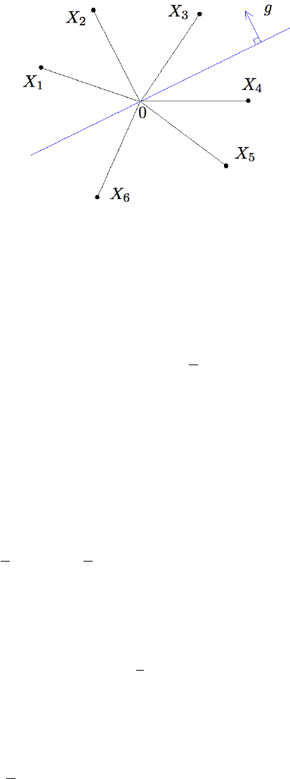
68 Random vectors in high dimensions
Figure 3.11 Randomized rounding of vectors X
i
∈ R
n
into labels x
i
= ±1.
For this configuration of points X
i
and a random hyperplane with normal
vector g, we assign x
1
= x
2
= x
3
= 1 and x
4
= x
5
= x
6
= −1.
Lemma 3.6.6 (Grothendieck’s identity). Consider a random vector g ∼ N(0, I
n
).
Then, for any fixed vectors u, v ∈ S
n−1
, we have
E sign ⟨g, u⟩sign ⟨g, v⟩ =
2
π
arcsin ⟨u, v⟩.
Exercise 3.6.7. KK Prove Grothendieck’s identity.
Hint: It will quickly follow once you show that the probability that ⟨g, u⟩ and ⟨g, v⟩ have opposite
signs equals α/π, where α ∈ [0, π] is the angle between the vectors u and v. To check this, use rotation
invariance to reduce the problem to R
2
. Once on the plane, rotation invariance will give the result.
A weak point of Grothendieck’s identity is the non-linear function arcsin, which
would be hard to work with. Let us replace it with a linear function using the
numeric inequality
1 −
2
π
arcsin t =
2
π
arccos t ≥ 0.878(1 − t), t ∈ [−1, 1], (3.27)
which can be easily verified using software; see Figure 3.12.
Proof of Theorem 3.6.5 By (3.23) and linearity of expectation, we have
E CUT(G, x) =
1
4
n
X
i,j=1
A
ij
(1 − E x
i
x
j
).
The definition of labels x
i
in the rounding step (3.26) gives
1 − E x
i
x
j
= 1 − E sign ⟨X
i
, g⟩sign
X
j
, g
= 1 −
2
π
arcsin
X
i
, X
j
(by Grothendieck’s identity, Lemma 3.6.6)
≥ 0.878(1 −
X
i
, X
j
) (by (3.27)).

3.7 Kernel trick, and tightening of Grothendieck’s inequality 69
-1 0 1
0
1
2
0.878(1 − t)
2
π
arccos t
Figure 3.12 The inequality
2
π
arccos t ≥ 0.878(1 −t) holds for all t ∈ [−1, 1].
Therefore
E CUT(G, x) ≥ 0.878 ·
1
4
n
X
i,j=1
A
ij
(1 −
X
i
, X
j
) = 0.878 SDP(G).
This proves the first inequality in the theorem. The second inequality is trivial
since SDP(G) ≥ MAX-CUT(G). (Why?)
3.7 Kernel trick, and tightening of Grothendieck’s inequality
Our proof of Grothendieck’s inequality given in Section 3.5 yields a very loose
bound on the absolute constant K. We now give an alternative proof that gives
(almost) the best known constant K ≤ 1.783.
Our new argument will be based on Grothendieck’s identity (Lemma (3.6.6)).
The main challenge in using this identity arises from the non-linearity of the
function arcsin(x). Indeed, suppose there were no such nonlinearity, and we hypo-
thetically had E sign ⟨g, u⟩sign ⟨g, v⟩ =
2
π
⟨u, v⟩. Then Grothendieck’s inequality
would easily follow:
2
π
X
i,j
a
ij
u
i
, v
j
=
X
i,j
a
ij
E sign ⟨g, u
i
⟩sign
g, v
j
≤ 1,
where in the last step we swapped the sum and expectation and used the assump-
tion of Grothendieck’s inequality with x
i
= sign ⟨g, u
i
⟩ and y
j
= sign
g, y
j
. This
would give Grothendieck’s inequality with K ≤ π/2 ≈ 1.57.
This argument is of course wrong. To address the non-linear form
2
π
arcsin ⟨u, v⟩
that appears in Grothendieck’s identity, we use the following remarkably powerful
trick: represent
2
π
arcsin ⟨u, v⟩ as the (linear) inner product ⟨u
′
, v
′
⟩ of some other
70 Random vectors in high dimensions
vectors u
′
, v
′
in some Hilbert space H. In the literature on machine learning, this
method is called the kernel trick.
We will explicitly construct the non-linear transformations u
′
= Φ(u), v
′
=
Ψ(v) that will do the job. Our construction is convenient to describe in the
language of tensors, which are a higher dimensional generalization of the notion
of matrices.
Definition 3.7.1 (Tensors). A tensor can be described as a multidimensional
array. Thus, a k-th order tensor (a
i
1
...i
k
) is a k-dimensional array of real numbers
a
i
1
...i
k
. The canonical inner product on R
n
1
×···×n
k
defines the inner product of
tensors A = (a
i
1
...i
k
) and B = (b
i
1
...i
k
):
⟨A, B⟩
:
=
X
i
1
,...,i
k
a
i
1
...i
k
b
i
1
...i
k
. (3.28)
Example 3.7.2. Scalars, vectors and matrices are examples of tensors. As we
noted in (3.19), for m ×n matrices the inner product of tensors (3.28) specializes
to
⟨A, B⟩ = tr(A
T
B) =
m
X
i=1
n
X
j=1
A
ij
B
ij
.
Example 3.7.3 (Rank-one tensors). Every vector u ∈ R
n
defines the k-th order
tensor product u ⊗ ··· ⊗ u, which is the tensor whose entries are the products of
all k-tuples of the entries of u. In other words,
u ⊗ ··· ⊗ u = u
⊗k
:
= (u
i
1
···u
i
k
) ∈ R
n×···×n
.
In particular, for k = 2, the tensor product u ⊗ u is just the n × n matrix which
is the outer product of u with itself:
u ⊗ u = (u
i
u
j
)
n
i,j=1
= uu
T
.
One can similarly define the tensor products u ⊗v ⊗··· ⊗ z for different vectors
u, v, . . . , z.
Exercise 3.7.4. K Show that for any vectors u, v ∈ R
n
and k ∈ N, we have
D
u
⊗k
, v
⊗k
E
= ⟨u, v⟩
k
.
This exercise shows a remarkable fact: we can represent non-linear forms like
⟨u, v⟩
k
as the usual, linear inner product in some other space. Formally, there
exist a Hilbert space H and a transformation Φ
:
R
n
→ H such that
Φ(u), Φ(v)
= ⟨u, v⟩
k
.
In this case, H is the space of k-th order tensors, and Φ(u) = u
⊗k
.
In the next two exercises, we extend this observation to more general non-
linearities.
Exercise 3.7.5. KK

3.7 Kernel trick, and tightening of Grothendieck’s inequality 71
(a) Show that there exist a Hilbert space H and a transformation Φ
:
R
n
→ H
such that
Φ(u), Φ(v)
= 2 ⟨u, v⟩
2
+ 5 ⟨u, v⟩
3
for all u, v ∈ R
n
.
Hint: Consider the cartesian product H = R
n×n
⊕ R
n×n×n
.
(b) More generally, consider a polynomial f
:
R → R with non-negative coeffi-
cients, and construct H and Φ such that
Φ(u), Φ(v)
= f(⟨u, v⟩) for all u, v ∈ R
n
.
(c) Show the same for any real analytic function f
:
R → R with non-negative
coefficients, i.e. for any function that can be represented as a convergent
series
f(x) =
∞
X
k=0
a
k
x
k
, x ∈ R, (3.29)
and such that a
k
≥ 0 for all k.
Exercise 3.7.6. K Let f
:
R → R be any real analytic function (with possibly
negative coefficients in (3.29)). Show that there exist a Hilbert space H and
transformations Φ, Ψ
:
R
n
→ H such that
Φ(u), Ψ(v)
= f(⟨u, v⟩) for all u, v ∈ R
n
.
Moreover, check that
∥Φ(u)∥
2
= ∥Ψ(u)∥
2
=
∞
X
k=0
|a
k
|∥u∥
2k
2
.
Hint: Construct Φ as in Exercise 3.7.5 with Φ, but include the signs of a
k
in the definition of Ψ.
Let us specialize the kernel trick to the non-linearity
2
π
arcsin ⟨u, v⟩ that appears
in Grothendieck’s identity.
Lemma 3.7.7. There exists a Hilbert space H and transformations
7
Φ, Ψ
:
S
n−1
→ S(H) such that
2
π
arcsin
Φ(u), Ψ(v)
= β ⟨u, v⟩ for all u, v ∈ S
n−1
, (3.30)
where β =
2
π
ln(1 +
√
2).
Proof Rewrite the desired identity (3.30) as
Φ(u), Ψ(v)
= sin
βπ
2
⟨u, v⟩
. (3.31)
The result of Exercise 3.7.6 gives us the Hilbert space H and the maps Φ, Ψ
:
7
Here S(H) denotes the unit sphere of the Hilbert space H.

72 Random vectors in high dimensions
R
n
→ H that satisfy (3.31). It only remains to determine the value of β for which
Φ and Ψ map unit vectors to unit vectors. To do this, we recall the Taylor series
sin t = t −
t
3
3!
+
t
5
5!
− ··· and sinh t = t +
t
3
3!
+
t
5
5!
+ ···
Exercise 3.7.6 then guarantees that for every u ∈ S
n−1
, we have
∥Φ(u)∥
2
= ∥Ψ(u)∥
2
= sinh
βπ
2
.
This quantity equals 1 if we set
β
:
=
2
π
arcsinh(1) =
2
π
ln(1 +
√
2).
The lemma is proved.
Now we are ready to prove Grothendieck’s inequality (Theorem 3.5.1) with
constant
K ≤
1
β
=
π
2 ln(1 +
√
2)
≈ 1.783.
Proof of Theorem 3.5.1 We can assume without loss of generality that u
i
, v
j
∈
S
N−1
(this is the same reduction as we did in the proof in Section 3.5). Lemma 3.7.7
gives us unit vectors u
′
i
= Φ(u
i
) and v
′
j
= Ψ(v
j
) in some Hilbert space H, which
satisfy
2
π
arcsin
D
u
′
i
, v
′
j
E
= β
u
i
, v
j
for all i, j.
We can again assume without loss of generality that H = R
M
for some M . (Why?)
Then
β
X
i,j
a
ij
u
i
, v
j
=
X
i,j
a
ij
·
2
π
arcsin
D
u
′
i
, v
′
j
E
=
X
i,j
a
ij
E sign
g, u
′
i
sign
D
g, v
′
j
E
(by Lemma 3.6.6),
≤ 1,
where in the last step we swapped the sum and expectation and used the assump-
tion of Grothendieck’s inequality with x
i
= sign ⟨g, u
′
i
⟩ and y
j
= sign
D
g, y
′
j
E
. This
yields the conclusion of Grothendieck’s inequality for K ≤ 1/β.
3.7.1 Kernels and feature maps
Since the kernel trick was so successful in the proof of Grothendieck’s inequality,
we may ask – what other non-linearities can be handled with the kernel trick?
Let
K
:
X × X → R

3.8 Notes 73
be a function of two variables on a set X. Under what conditions on K can we
find a Hilbert space H and a transformation
Φ
:
X → H
so that
Φ(u), Φ(v)
= K(u, v) for all u, v ∈ X? (3.32)
The answer to this question is provided by Mercer’s and, more precisely, Moore-
Aronszajn’s theorems. The necessary and sufficient condition is that K be a
positive semidefinite kernel, which means that for any finite collection of points
u
1
, . . . , u
N
∈ X, the matrix
K(u
i
, u
j
)
N
i,j=1
is symmetric and positive semidefinite. The map Φ is called a feature map, and the
Hilbert space H can be constructed from the kernel K as a (unique) reproducing
kernel Hilbert space.
Examples of positive semidefinite kernels on R
n
that are common in machine
learning include the Gaussian kernel (also called the radial basis function kernel)
K(u, v) = exp
−
∥u − v∥
2
2
2σ
2
, u, v ∈ R
n
, σ > 0
and the polynomial kernel
K(u, v) =
⟨u, v⟩+ r
k
, u, v ∈ R
n
, r > 0, k ∈ N.
The kernel trick (3.32), which represents a general kernel K(u, v) as an inner
product, is very popular in machine learning. It allows one to handle non-linear
models (determined by kernels K) by using methods developed for linear models.
In contrast to what we did in this section, in machine learning applications the
explicit description of the Hilbert space H and the feature map Φ
:
X → H is
typically not needed. Indeed, to compute the inner product
Φ(u), Φ(v)
in H,
one does not need to know Φ: the identity (3.32) allows one to compute K(u, v)
instead.
3.8 Notes
Theorem 3.1.1 about the concentration of the norm of random vectors is known
but difficult to locate in the existing literature. We will later prove a more gen-
eral result, Theorem 6.3.2, which is valid for anisotropic random vectors. It is
unknown if the quadratic dependence on K in Theorem 3.1.1 is optimal. One
may also wonder about concentration of the norm ∥X∥
2
of random vectors X
whose coordinates are not necessarily independent. In particular, for a random
vector X that is uniformly distributed in a convex set K, concentration of the
norm is one of the central problems in geometric functional analysis; see [93,
Section 2] and [36, Chapter 12].

74 Random vectors in high dimensions
Exercise 3.3.4 mentions Cram´er-Wold’s theorem. It a straightforward conse-
quence of the uniqueness theorem for characteristic functions, see [23, Section 29].
The concept of frames introduced in Section 3.3.4 is an important extension
of the notion of orthogonal bases. One can read more about frames and their
applications in signal processing and data compression e.g. in [51, 121].
Sections 3.3.5 and 3.4.4 discuss random vectors uniformly distributed in con-
vex sets. The books [11, 36] study this topic in detail, and the surveys [185, 218]
discuss algorithmic aspects of computing the volume of convex sets in high di-
mensions.
Our discussion of sub-gaussian random vectors in Section 3.4. mostly follows
[222]. An alternative geometric proof of Theorem 3.4.6 can be found in [13,
Lemma 2.2].
Grothendieck’s inequality (Theorem 3.5.1) was originally proved by A. Gro-
thendieck in 1953 [90] with bound on the constant K ≤ sinh(π/2) ≈ 2.30; a
version of this original argument is presented [133, Section 2]. There is a number
of alternative proofs of Grothendieck’s inequality with better and worse bounds
on K; see [35] for the history. The surveys [115, 168] discuss ramifications and
applications of Grothendieck’s inequality in various areas of mathematics and
computer science. Our first proof of Grothendieck’s inequality, the one given
in Section 3.5, is similar to the one in [5, Section 8.1]; it was kindly brought to
author’s attention by Mark Rudelson. Our second proof, the one from Section 3.7,
is due to J.-L. Krivine [122]; versions of this argument can be found e.g. in [7]
and [126]. The bound on the constant K ≤
π
2 ln(1+
√
2)
≈ 1.783 that follows from
Krivine’s argument is currently the best known explicit bound on K. It has been
proved, however, that the best possible bound must be strictly smaller than
Krivine’s bound, but no explicit number is known [35].
A part of this chapter is about semidefinite relaxations of hard optimiza-
tion problems. For an introduction to the area of convex optimization, including
semidefinite programming, we refer to the books [34, 39, 126, 29]. For the use of
Grothendieck’s inequality in analyzing semidefinite relaxations, see [115, 7]. Our
presentation of the maximum cut problem in Section 3.6 follows [39, Section 6.6]
and [126, Chapter 7]. The semidefinite approach to maximum cut, which we dis-
cussed in Section 3.6.3, was pioneered in 1995 by M. Goemans and D. Williamson
[83]. The approximation ratio
2
π
min
0≤θ≤π
θ
1−cos(θ)
≈ 0.878 guaranteed by the
Goemans-Williamson algorithm remains the best known constant for the max-cut
problem. If the Unique Games Conjecture is true, this ratio can not be improved,
i.e. any better approximation would be NP-hard to compute [114].
In Section 3.7 we give Krivine’s proof of Grothendieck’s inequality [122]. We
also briefly discuss kernel methods there. To learn more about kernels, reproduc-
ing kernel Hilbert spaces and their applications in machine learning, see e.g. the
survey [102].

4
Random matrices
We begin to study the non-asymptotic theory of random matrices, a study that
will be continued in many further chapters. Section 4.1 is a quick reminder about
singular values and matrix norms and their relationships. Section 4.2 introduces
important geometric concepts – nets, covering and packing numbers, metric en-
tropy, and discusses relations of these quantities with volume and coding. In
Sections 4.4 and 4.6, we develop a basic ε-net argument and use it for random
matrices. We first give a bound on the operator norm (Theorem 4.4.5) and then a
stronger, two-sided bound on all singular values (Theorem 4.6.1) of random ma-
trices. Three applications of random matrix theory are discussed in this chapter:
a spectral clustering algorithm for recovering clusters, or communities, in com-
plex networks (Section 4.5), covariance estimation (Section 4.7) and a spectral
clustering algorithm for data presented as geometric point sets (Section 4.7.1).
4.1 Preliminaries on matrices
You should be familiar with the notion of singular value decomposition from a
basic course in linear algebra; we recall it nevertheless. We will then introduce
two matrix norms – operator and Frobenius, and discuss their relationships.
4.1.1 Singular value decomposition
The main object of our study will be an m ×n matrix A with real entries. Recall
that A can be represented using the singular value decomposition (SVD), which
we can write as
A =
r
X
i=1
s
i
u
i
v
T
i
, where r = rank(A). (4.1)
Here the non-negative numbers s
i
= s
i
(A) are called singular values of A, the
vectors u
i
∈ R
m
are called the left singular vectors of A, and the vectors v
i
∈ R
n
are called the right singular vectors of A.
For convenience, we often extend the sequence of singular values by setting
s
i
= 0 for r < i ≤ n, and we arrange them in a non-increasing order:
s
1
≥ s
2
≥ ··· ≥ s
n
≥ 0.
The left singular vectors u
i
are the orthonormal eigenvectors of AA
T
and the
75

76 Random matrices
right singular vectors v
i
are the orthonormal eigenvectors of A
T
A. The singular
values s
i
are the square roots of the eigenvalues λ
i
of both AA
T
and A
T
A:
s
i
(A) =
q
λ
i
(AA
T
) =
q
λ
i
(A
T
A).
In particular, if A is a symmetric matrix, then the singular values of A are the
absolute values of the eigenvalues λ
i
of A:
s
i
(A) = |λ
i
(A)|,
and both left and right singular vectors of A are eigenvectors of A.
Courant-Fisher’s min-max theorem offers the following variational characteri-
zation of eigenvalues λ
i
(A) of a symmetric matrix A, assuming they are arranged
in a non-increasing order:
λ
i
(A) = max
dim E=i
min
x∈S(E)
⟨Ax, x⟩, (4.2)
Here the maximum is over all i-dimensional subspaces E of R
n
, and the minimum
is over all unit vectors x ∈ E, and S(E) denotes the unit Euclidean sphere in the
subspace E. For the singular values, the min-max theorem immediately implies
that
s
i
(A) = max
dim E=i
min
x∈S(E)
∥Ax∥
2
.
Exercise 4.1.1. K Suppose A is an invertible matrix with singular value de-
composition
A =
n
X
i=1
s
i
u
i
v
T
i
.
Check that
A
−1
=
n
X
i=1
1
s
i
v
i
u
T
i
.
4.1.2 Operator norm and the extreme singular values
The space of m × n matrices can be equipped with several classical norms. We
mention two of them – operator and Frobenius norms – and emphasize their
connection with the spectrum of A.
When we think of the space R
m
along with the Euclidean norm ∥ · ∥
2
on it,
we denote this Hilbert space ℓ
m
2
. The matrix A acts as a linear operator from
ℓ
n
2
→ ℓ
m
2
. Its operator norm, also called the spectral norm, is defined as
∥A∥
:
= ∥A
:
ℓ
n
2
→ ℓ
m
2
∥ = max
x∈R
n
\{0}
∥Ax∥
2
∥x∥
2
= max
x∈S
n−1
∥Ax∥
2
.
Equivalently, the operator norm of A can be computed by maximizing the quadratic
form ⟨Ax, y⟩ over all unit vectors x, y:
∥A∥ = max
x∈S
n−1
, y∈S
m−1
⟨Ax, y⟩.

4.1 Preliminaries on matrices 77
In terms of spectrum, the operator norm of A equals the largest singular value
of A:
s
1
(A) = ∥A∥.
(Check!)
The smallest singular value s
n
(A) also has a special meaning. By definition,
it can only be non-zero for tall matrices where m ≥ n. In this case, A has full
rank n if and only if s
n
(A) > 0. Moreover, s
n
(A) is a quantitative measure of
non-degeneracy of A. Indeed, if A has full rank then
s
n
(A) =
1
∥A
+
∥
where A
+
is the Moore-Penrose pseudoinverse of A. Its norm ∥A
+
∥ is the norm
of the operator A
−1
restricted to the image of A.
4.1.3 Frobenius norm
The Frobenius norm, also called Hilbert-Schmidt norm of a matrix A with entries
A
ij
is defined as
∥A∥
F
=
m
X
i=1
n
X
j=1
|A
ij
|
2
1/2
.
Thus the Frobenius norm is the Euclidean norm on the space of matrices R
m×n
.
In terms of singular values, the Frobenius norm can be computed as
∥A∥
F
=
r
X
i=1
s
i
(A)
2
1/2
.
The canonical inner product on R
m×n
can be represented in terms of matrices as
⟨A, B⟩ = tr(A
T
B) =
m
X
i=1
n
X
j=1
A
ij
B
ij
. (4.3)
Obviously, the canonical inner product generates the canonical Euclidean norm,
i.e.
∥A∥
2
F
= ⟨A, A⟩.
Let us now compare the operator and the Frobenius norm. If we look at the
vector s = (s
1
, . . . , s
r
) of singular values of A, these norms become the ℓ
∞
and ℓ
2
norms, respectively:
∥A∥ = ∥s∥
∞
, ∥A∥
F
= ∥s∥
2
.
Using the inequality ∥s∥
∞
≤ ∥s∥
2
≤
√
r ∥s∥
∞
for s ∈ R
n
(check it!) we obtain the
best possible relation between the operator and Frobenius norms:
∥A∥ ≤ ∥A∥
F
≤
√
r ∥A∥. (4.4)

78 Random matrices
Exercise 4.1.2. KK Prove the following bound on the singular values s
i
of
any matrix A:
s
i
≤
1
√
i
∥A∥
F
.
4.1.4 Low-rank approximation
Suppose we want to approximate a given matrix A of rank r by a matrix A
k
that
has a given lower rank, say rank k < r. What is the best choice for A
k
? In other
words, what matrix A
k
of rank k minimizes the distance to A? The distance can
be measured by the operator norm or Frobenius norm.
In either case, Eckart-Young-Mirsky’s theorem gives the answer to the low-rank
approximation problem. It states that the minimizer A
k
is obtained by truncating
the singular value decomposition of A at the k-th term:
A
k
=
k
X
i=1
s
i
u
i
v
T
i
.
In other words, the Eckart-Young-Mirsky theorem states that
∥A − A
k
∥ = min
rank(A
′
)≤k
∥A − A
′
∥.
A similar statement holds for the Frobenius norm (and, in fact, for any unitary-
invariant norm). The matrix A
k
is often called the best rank k approximation of
A.
Exercise 4.1.3 (Best rank k approximation). KK Let A
k
be the best rank k
approximation of a matrix A. Express ∥A −A
k
∥
2
and ∥A −A
k
∥
2
F
in terms of the
singular values s
i
of A.
4.1.5 Approximate isometries
The extreme singular values s
1
(A) and s
n
(A) have an important geometric mean-
ing. They are respectively the smallest number M and the largest number m that
make the following inequality true:
m∥x∥
2
≤ ∥Ax∥
2
≤ M∥x∥
2
for all x ∈ R
n
. (4.5)
(Check!) Applying this inequality for x−y instead of x and with the best bounds,
we can rewrite it as
s
n
(A)∥x − y∥
2
≤ ∥Ax − Ay∥
2
≤ s
1
(A)∥x − y∥
2
for all x ∈ R
n
.
This means that the matrix A, acting as an operator from R
n
to R
m
, can only
change the distance between any points by a factor that lies between s
n
(A) and
s
1
(A). Thus the extreme singular values control the distortion of the geometry of
R
n
under the action of A.
The best possible matrices in this sense, which preserve distances exactly, are

4.1 Preliminaries on matrices 79
called isometries. Let us recall their characterization, which can be proved using
elementary linear algebra.
Exercise 4.1.4 (Isometries). K Let A be an m ×n matrix with m ≥ n. Prove
that the following statements are equivalent.
(a) A
T
A = I
n
.
(b) P
:
= AA
T
is an orthogonal projection
1
in R
m
onto a subspace of dimension
n.
(c) A is an isometry, or isometric embedding of R
n
into R
m
, which means that
∥Ax∥
2
= ∥x∥
2
for all x ∈ R
n
.
(d) All singular values of A equal 1; equivalently
s
n
(A) = s
1
(A) = 1.
Quite often the conditions of Exercise 4.1.4 hold only approximately, in which
case we regard A as an approximate isometry.
Lemma 4.1.5 (Approximate isometries). Let A be an m × n matrix and δ > 0.
Suppose that
∥A
T
A − I
n
∥ ≤ max(δ, δ
2
).
Then
(1 − δ)∥x∥
2
≤ ∥Ax∥
2
≤ (1 + δ)∥x∥
2
for all x ∈ R
n
. (4.6)
Consequently, all singular values of A are between 1 − δ and 1 + δ:
1 − δ ≤ s
n
(A) ≤ s
1
(A) ≤ 1 + δ. (4.7)
Proof To prove (4.6), we may assume without loss of generality that ∥x∥
2
= 1.
(Why?) Then, using the assumption, we get
max(δ, δ
2
) ≥
D
(A
T
A − I
n
)x, x
E
=
∥Ax∥
2
2
− 1
.
Applying the elementary inequality
max(|z − 1|, |z − 1|
2
) ≤ |z
2
− 1|, z ≥ 0 (4.8)
for z = ∥Ax∥
2
, we conclude that
∥Ax∥
2
− 1
≤ δ.
This proves (4.6), which in turn implies (4.7) as we saw in the beginning of this
section.
Exercise 4.1.6 (Approximate isometries). KK Prove the following converse to
Lemma 4.1.5: if (4.7) holds, then
∥A
T
A − I
n
∥ ≤ 3 max(δ, δ
2
).
1
Recall that P is a projection if P
2
= P , and P is called orthogonal if the image and kernel of P are
orthogonal subspaces.
80 Random matrices
Remark 4.1.7 (Projections vs. isometries). Consider an n ×m matrix Q. Then
QQ
T
= I
n
if and only if
P
:
= Q
T
Q
is an orthogonal projection in R
m
onto a subspace of dimension n. (This can be
checked directly or deduced from Exercise 4.1.4 by taking A = Q
T
.) In case this
happens, the matrix Q itself is often called a projection from R
m
onto R
n
.
Note that A is an isometric embedding of R
n
into R
m
if and only if A
T
is a
projection from R
m
onto R
n
. These remarks can be also made for an approximate
isometry A; the transpose A
T
in this case is an approximate projection.
Exercise 4.1.8 (Isometries and projections from unitary matrices). K Canon-
ical examples of isometries and projections can be constructed from a fixed uni-
tary matrix U. Check that any sub-matrix of U obtained by selecting a subset
of columns is an isometry, and any sub-matrix obtained by selecting a subset of
rows is a projection.
4.2 Nets, covering numbers and packing numbers
We are going to develop a simple but powerful method – an ε-net argument –
and illustrate its usefulness for the analysis of random matrices. In this section,
we recall the concept of an ε-net, which you may have seen in a course in real
analysis, and we relate it to some other basic notions – covering, packing, entropy,
volume, and coding.
Definition 4.2.1 (ε-net). Let (T, d) be a metric space. Consider a subset K ⊂ T
and let ε > 0. A subset N ⊆ K is called an ε-net of K if every point in K is
within distance ε of some point of N, i.e.
∀x ∈ K ∃x
0
∈ N
:
d(x, x
0
) ≤ ε.
Equivalently, N is an ε-net of K if and only if K can be covered by balls with
centers in N and radii ε, see Figure 4.1a.
If you ever feel confused by too much generality, it might be helpful to keep in
mind an important example. Let T = R
n
with d being the Euclidean distance,
i.e.
d(x, y) = ∥x − y∥
2
, x, y ∈ R
n
. (4.9)
In this case, we cover a subset K ⊂ R
n
by round balls, as shown in Figure 4.1a.
We already saw an example of such covering in Corollary 0.0.4 where K was a
polytope.
Definition 4.2.2 (Covering numbers). The smallest possible cardinality of an
ε-net of K is called the covering number of K and is denoted N(K, d, ε). Equiv-
alently, N(K, d, ε) is the smallest number of closed balls with centers in K and
radii ε whose union covers K.

4.2 Nets, covering numbers and packing numbers 81
(a) This covering of a pentagon K by seven ε-
balls shows that N(K, ε) ≤ 7.
(b) This packing of a pentagon K by ten ε/2-
balls shows that P(K, ε) ≥ 10.
Figure 4.1 Packing and covering
Remark 4.2.3 (Compactness). An important result in real analysis states that
a subset K of a complete metric space (T, d) is precompact (i.e. the closure of K
is compact) if and only if
N(K, d, ε) < ∞ for every ε > 0.
Thus we can think about the magnitude N(K, d, ε) as a quantitative measure of
compactness of K.
Closely related to covering is the notion of packing.
Definition 4.2.4 (Packing numbers). A subset N of a metric space (T, d) is
ε-separated if d(x, y) > ε for all distinct points x, y ∈ N. The largest possible
cardinality of an ε-separated subset of a given set K ⊂ T is called the packing
number of K and is denoted P(K, d, ε).
Exercise 4.2.5 (Packing the balls into K). KK
(a) Suppose T is a normed space. Prove that P(K, d, ε) is the largest number
of closed disjoint balls with centers in K and radii ε/2. See Figure 4.1b for
an illustration.
(b) Show by example that the previous statement may be false for a general
metric space T .
Lemma 4.2.6 (Nets from separated sets). Let N be a maximal
2
ε-separated
subset of K. Then N is an ε-net of K.
Proof Let x ∈ K; we want to show that there exists x
0
∈ N such that d(x, x
0
) ≤
ε. If x ∈ N, the conclusion is trivial by choosing x
0
= x. Suppose now x ̸∈ N.
The maximality assumption implies that N ∪ {x} is not ε-separated. But this
means precisely that d(x, x
0
) ≤ ε for some x
0
∈ N.
Remark 4.2.7 (Constructing a net). Lemma 4.2.6 leads to the following simple
algorithm for constructing an ε-net of a given set K. Choose a point x
1
∈ K
2
Here by “maximal” we mean that adding any new point to N destroys the separation property.

82 Random matrices
arbitrarily, choose a point x
2
∈ K which is farther than ε from x
1
, choose x
3
so
that it is farther than ε from both x
1
and x
2
, and so on. If K is compact, the
algorithm terminates in finite time (why?) and gives an ε-net of K.
The covering and packing numbers are essentially equivalent:
Lemma 4.2.8 (Equivalence of covering and packing numbers). For any set K ⊂
T and any ε > 0, we have
P(K, d, 2ε) ≤ N(K, d, ε) ≤ P(K, d, ε).
Proof The upper bound follows from Lemma 4.2.6. (How?)
To prove the lower bound, choose an 2ε-separated subset P = {x
i
} in K and
an ε-net N = {y
j
} of K. By the definition of a net, each point x
i
belongs a
closed ε-ball centered at some point y
j
. Moreover, since any closed ε-ball can not
contain a pair of 2ε-separated points, each ε-ball centered at y
j
may contain at
most one point x
i
. The pigeonhole principle then yields |P| ≤ |N|. Since this
happens for arbitrary packing P and covering N, the lower bound in the lemma
is proved.
Exercise 4.2.9 (Allowing the centers to be outside K). KKK In our definition
of the covering numbers of K, we required that the centers x
i
of the balls B(x
i
, ε)
that form a covering lie in K. Relaxing this condition, define the exterior covering
number N
ext
(K, d, ε) similarly but without requiring that x
i
∈ K. Prove that
N
ext
(K, d, ε) ≤ N(K, d, ε) ≤ N
ext
(K, d, ε/2).
Exercise 4.2.10 (Monotonicity). KKK Give a counterexample to the following
monotonicity property:
L ⊂ K implies N(L, d, ε) ≤ N(K, d, ε).
Prove an approximate version of monotonicity:
L ⊂ K implies N(L, d, ε) ≤ N(K, d, ε/2).
4.2.1 Covering numbers and volume
Let us now specialize our study of covering numbers to the most important ex-
ample where T = R
n
with the Euclidean metric
d(x, y) = ∥x − y∥
2
as in (4.9). To ease the notation, we often omit the metric when it is understood,
thus writing
N(K, ε) = N(K, d, ε).
If the covering numbers measure the size of K, how are they related to the
most classical measure of size, the volume of K in R
n
? There could not be a full
equivalence between these two quantities, since “flat” sets have zero volume but
non-zero covering numbers.
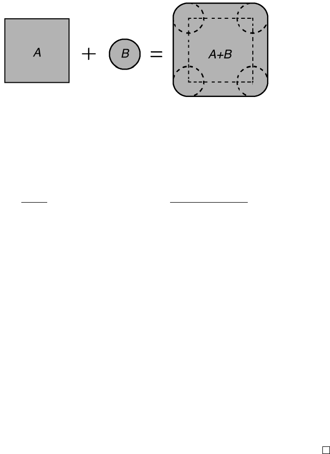
4.2 Nets, covering numbers and packing numbers 83
Still, there is a useful partial equivalence, which is often quite sharp. It is based
on the notion of Minkowski sum of sets in R
n
.
Definition 4.2.11 (Minkowski sum). Let A and B be subsets of R
n
. The Minkowski
sum A + B is defined as
A + B
:
= {a + b
:
a ∈ A, b ∈ B}.
Figure 4.2 shows an example of Minkowski sum of two sets on the plane.
Figure 4.2 Minkowski sum of a square and a circle is a square with
rounded corners.
Proposition 4.2.12 (Covering numbers and volume). Let K be a subset of R
n
and ε > 0. Then
|K|
|εB
n
2
|
≤ N(K, ε) ≤ P(K, ε) ≤
|(K + (ε/2)B
n
2
)|
|(ε/2)B
n
2
|
.
Here |·| denotes the volume in R
n
, B
n
2
denotes the unit Euclidean ball
3
in R
n
, so
εB
n
2
is a Euclidean ball with radius ε.
Proof The middle inequality follows from Lemma 4.2.8, so all we need to prove
is the left and right bounds.
(Lower bound) Let N
:
= N(K, ε). Then K can be covered by N balls with
radii ε. Comparing the volumes, we obtain
|K| ≤ N · |εB
n
2
|,
Dividing both sides by |εB
n
2
| yields the lower bound.
(Upper bound) Let N
:
= P(K, ε). Then one can construct N closed disjoint
balls B(x
i
, ε/2) with centers x
i
∈ K and radii ε/2 (see Exercise 4.2.5). While
these balls may not need to fit entirely in K (see Figure 4.1b), they do fit in a
slightly inflated set, namely K + (ε/2)B
n
2
. (Why?) Comparing the volumes, we
obtain
N · |(ε/2)B
n
2
| ≤ |K + (ε/2)B
n
2
|.
which leads to the upper bound in the proposition.
3
Thus B
n
2
= {x ∈ R
n
:
∥x∥
2
≤ 1}.

84 Random matrices
An important consequence of the volumetric bound (4.10) is that the covering
(and thus packing) numbers of the Euclidean ball, as well as many other sets, are
exponential in the dimension n. Let us check this.
Corollary 4.2.13 (Covering numbers of the Euclidean ball). The covering num-
bers of the unit Euclidean ball B
n
2
satisfy the following for any ε > 0:
1
ε
n
≤ N(B
n
2
, ε) ≤
2
ε
+ 1
n
.
The same upper bound is true for the unit Euclidean sphere S
n−1
.
Proof The lower bound follows immediately from Proposition 4.2.12, since the
volume in R
n
scales as
|εB
n
2
| = ε
n
|B
n
2
|.
The upper bound follows from Proposition 4.2.12, too:
N(B
n
2
, ε) ≤
|(1 + ε/2)B
n
2
|
|(ε/2)B
n
2
|
=
(1 + ε/2)
n
(ε/2)
n
=
2
ε
+ 1
n
.
The upper bound for the sphere can be proved in the same way.
To simplify the bound a bit, note that in the non-trivial range ε ∈ (0, 1] we
have
1
ε
n
≤ N(B
n
2
, ε) ≤
3
ε
n
. (4.10)
In the trivial range where ε > 1, the unit ball can be covered by just one ε-ball,
so N(B
n
2
, ε) = 1.
The volumetric argument we just gave works well in many other situations.
Let us give an important example.
Definition 4.2.14 (Hamming cube). The Hamming cube {0, 1}
n
consists of all
binary strings of length n. The Hamming distance d
H
(x, y) between two binary
strings is defined as the number of bits where x and y disagree, i.e.
d
H
(x, y)
:
= #
n
i
:
x(i) ̸= y(i)
o
, x, y ∈ {0, 1}
n
.
Endowed with this metric, the Hamming cube is a metric space ({0, 1}
n
, d
H
),
which is sometimes called the Hamming space.
Exercise 4.2.15. K Check that d
H
is indeed a metric.
Exercise 4.2.16 (Covering and packing numbers of the Hamming cube). KKK
Let K = {0, 1}
n
. Prove that for every integer m ∈ [0, n], we have
2
n
P
m
k=0
n
k
≤ N(K, d
H
, m) ≤ P(K, d
H
, m) ≤
2
n
P
⌊m/2⌋
k=0
n
k
Hint: Adapt the volumetric argument by replacing volume by cardinality.
To make these bounds easier to compute, one can use the bounds for binomial
sums from Exercise 0.0.5.

4.3 Application: error correcting codes 85
4.3 Application: error correcting codes
Covering and packing arguments frequently appear in applications to coding the-
ory. Here we give two examples that relate covering and packing numbers to
complexity and error correction.
4.3.1 Metric entropy and complexity
Intuitively, the covering and packing numbers measure the complexity of a set
K. The logarithm of the covering numbers log
2
N(K, ε) is often called the metric
entropy of K. As we will see now, the metric entropy is equivalent to the number
of bits needed to encode points in K.
Proposition 4.3.1 (Metric entropy and coding). Let (T, d) be a metric space,
and consider a subset K ⊂ T . Let C(K, d, ε) denote the smallest number of bits
sufficient to specify every point x ∈ K with accuracy ε in the metric d. Then
log
2
N(K, d, ε) ≤ C(K, d, ε) ≤
log
2
N(K, d, ε/2)
.
Proof (Lower bound) Assume C(K, d, ε) ≤ N . This means that there exists a
transformation (“encoding”) of points x ∈ K into bit strings of length N , which
specifies every point with accuracy ε. Such a transformation induces a partition of
K into at most 2
N
subsets, which are obtained by grouping the points represented
by the same bit string; see Figure 4.3 for an illustration. Each subset must have
diameter
4
at most ε, and thus it can be covered by a ball centered in K and with
radius ε. (Why?) Thus K can be covered by at most 2
N
balls with radii ε. This
implies that N(K, d, ε) ≤ 2
N
. Taking logarithms on both sides, we obtain the
lower bound in the proposition.
(Upper bound) Assume log
2
N(K, d, ε/2) ≤ N for some integer N . This
means that there exists an (ε/2)-net N of K with cardinality |N| ≤ 2
N
. To every
point x ∈ K, let us assign a point x
0
∈ N that is closest to x. Since there are at
most 2
N
such points, N bits are sufficient to specify the point x
0
. It remains to
note that the encoding x 7→ x
0
represents points in K with accuracy ε. Indeed,
if both x and y are encoded by the same x
0
then, by triangle inequality,
d(x, y) ≤ d(x, x
0
) + d(y, x
0
) ≤
ε
2
+
ε
2
= ε
This shows that C(K, d, ε) ≤ N . This completes the proof.
4.3.2 Error correcting codes
Suppose Alice wants to send Bob a message that consists of k letters, such as
x
:
= “fill the glass”.
4
If (T, d) is a metric space and K ⊂ T , the diameter of the set K is defined as
diam(K)
:
= sup{d(x, y)
:
x, y ∈ K}.

86 Random matrices
Figure 4.3 Encoding points in K as N -bit strings induces a partition of K
into at most 2
N
subsets.
Suppose further that an adversary may corrupt Alice’s message by changing at
most r letters in it. For example, Bob may receive
y
:
= “bill the class”
if r = 2. Is there a way to protect the communication channel between Alice and
Bob, a method that can correct adversarial errors?
A common approach relies on using redundancy. Alice would encode her k-
letter message into a longer, n-letter, message for some n > k, hoping that the
extra information would help Bob get her message right despite any r errors.
Example 4.3.2 (Repetition code). Alice may just repeat her message several
times, thus sending to Bob
E(x)
:
= “fill the glass fill the glass fill the glass fill the glass fill the glass”.
Bob could then use the majority decoding: to determine the value of any particular
letter, he would look at the received copies of it in E(x) and choose the value
that occurs most frequently. If the original message x is repeated 2r + 1 times,
then the majority decoding recovers x exactly even when r letters of E(x) are
corrupted. (Why?)
The problem with majority decoding is that it is very inefficient: it uses
n = (2r + 1)k (4.11)
letters to encode a k-letter message. As we will see shortly, there exist error
correcting codes with much smaller n.
But first let us formalize the notion of an error correcting code – an encoding
of k-letter strings into n-letter strings that can correct r errors. For convenience,
instead of using the English alphabet we shall work with the binary alphabet
consisting of two letters 0 and 1.
Definition 4.3.3 (Error correcting code). Fix integers k, n and r. Two maps
E
:
{0, 1}
k
→ {0, 1}
n
and D
:
{0, 1}
n
→ {0, 1}
k

4.3 Application: error correcting codes 87
are called encoding and decoding maps that can correct r errors if we have
D(y) = x
for every word x ∈ {0, 1}
k
and every string y ∈ {0, 1}
n
that differs from E(x) in
at most r bits. The encoding map E is called an error correcting code; its image
E({0, 1}
k
) is called a codebook (and very often the image itself is called the error
correcting code); the elements E(x) of the image are called codewords.
We now relate error correction to packing numbers of the Hamming cube
({0, 1}
n
, d
H
) where d
H
is the Hamming metric we introduced in Definition 4.2.14.
Lemma 4.3.4 (Error correction and packing). Assume that positive integers k,
n and r are such that
log
2
P({0, 1}
n
, d
H
, 2r) ≥ k.
Then there exists an error correcting code that encodes k-bit strings into n-bit
strings and can correct r errors.
Proof By assumption, there exists a subset N ⊂ {0, 1}
n
with cardinality |N| =
2
k
and such that the closed balls centered at the points in N and with radii r
are disjoint. (Why?) We then define the encoding and decoding maps as follows:
choose E
:
{0, 1}
k
→ N to be an arbitrary one-to-one map and D
:
{0, 1}
n
→
{0, 1}
k
to be a nearest neighbor decoder.
5
Now, if y ∈ {0, 1}
n
differs from E(x) in at most r bits, y lies in the closed ball
centered at E(x) and with radius r. Since such balls are disjoint by construction,
y must be strictly closer to E(x) than to any other codeword E(x
′
) in N. Thus
the nearest-neighbor decoding decodes y correctly, i.e. D(y) = x. This completes
the proof.
Let us substitute into Lemma 4.3.4 the bounds on the packing numbers of the
Hamming cube from Exercise 4.2.16.
Theorem 4.3.5 (Guarantees for an error correcting code). Assume that positive
integers k, n and r are such that
n ≥ k + 2r log
2
en
2r
.
Then there exists an error correcting code that encodes k-bit strings into n-bit
strings and can correct r errors.
Proof Passing from packing to covering numbers using Lemma 4.2.8 and then
using the bounds on the covering numbers from Exercises 4.2.16 (and simplifying
using Exercise 0.0.5), we get
P({0, 1}
n
, d
H
, 2r) ≥ N({0, 1}
n
, d
H
, 2r) ≥ 2
n
2r
en
2r
.
5
Formally, we set D(y) = x
0
where E(x
0
) is the closest codeword in N to y; break ties arbitrarily.

88 Random matrices
By assumption, this quantity is further bounded below by 2
k
. An application of
Lemma 4.3.4 completes the proof.
Informally, Theorem 4.3.5 shows that we can correct r errors if we make the
information overhead n − k almost linear in r:
n − k ≍ r log
n
r
.
This overhead is much smaller than for the repetition code (4.11). For example,
to correct two errors in Alice’s twelve-letter message “fill the glass”, encoding it
into a 30-letter codeword would suffice.
Remark 4.3.6 (Rate). The guarantees of a given error correcting code are tradi-
tionally expressed in terms of the tradeoff between the rate and fraction of errors,
defined as
R
:
=
k
n
and δ
:
=
r
n
.
Theorem 4.3.5 states that there exist error correcting codes with rate as high as
R ≥ 1 − f(2δ)
where f(t) = t log
2
(e/t).
Exercise 4.3.7 (Optimality). KKK
(a) Prove the converse to the statement of Lemma 4.3.4.
(b) Deduce a converse to Theorem 4.3.5. Conclude that for any error correcting
code that encodes k-bit strings into n-bit strings and can correct r errors,
the rate must be
R ≤ 1 − f(δ)
where f(t) = t log
2
(1/t) as before.
4.4 Upper bounds on random sub-gaussian matrices
We are now ready to begin to study the non-asymptotic theory of random ma-
trices. Random matrix theory is concerned with m × n matrices A with random
entries. The central questions of this theory are about the distributions of singular
values, eigenvalues (if A is symmetric) and eigenvectors of A.
Theorem 4.4.5 will give a first bound on the operator norm (equivalently, on
the largest singular value) of a random matrix with independent sub-gaussian
entries. It is neither the sharpest nor the most general result; it will be sharpened
and extended in Sections 4.6 and 6.5.
But before we do this, let us pause to learn how ε-nets can help us compute
the operator norm of a matrix.

4.4 Upper bounds on random sub-gaussian matrices 89
4.4.1 Computing the norm on a net
The notion of ε-nets can help us to simplify various problems involving high-
dimensional sets. One such problem is the computation of the operator norm of
an m × n matrix A. The operator norm was defined in Section 4.1.2 as
∥A∥ = max
x∈S
n−1
∥Ax∥
2
.
Thus, to evaluate ∥A∥ one needs to control ∥Ax∥ uniformly over the sphere S
n−1
.
We will show that instead of the entire sphere, it is enough to gain control just
over an ε-net of the sphere (in the Euclidean metric).
Lemma 4.4.1 (Computing the operator norm on a net). Let A be an m × n
matrix and ε ∈ [0, 1). Then, for any ε-net N of the sphere S
n−1
, we have
sup
x∈N
∥Ax∥
2
≤ ∥A∥ ≤
1
1 − ε
· sup
x∈N
∥Ax∥
2
Proof The lower bound in the conclusion is trivial since N ⊂ S
n−1
. To prove
the upper bound, fix a vector x ∈ S
n−1
for which
∥A∥ = ∥Ax∥
2
and choose x
0
∈ N that approximates x so that
∥x − x
0
∥
2
≤ ε.
By the definition of the operator norm, this implies
∥Ax − Ax
0
∥
2
= ∥A(x − x
0
)∥
2
≤ ∥A∥∥x − x
0
∥
2
≤ ε∥A∥.
Using triangle inequality, we find that
∥Ax
0
∥
2
≥ ∥Ax∥
2
− ∥Ax − Ax
0
∥
2
≥ ∥A∥ − ε∥A∥ = (1 − ε)∥A∥.
Dividing both sides of this inequality by 1 − ε, we complete the proof.
Exercise 4.4.2. K Let x ∈ R
n
and N be an ε-net of the sphere S
n−1
. Show
that
sup
y∈N
⟨x, y⟩ ≤ ∥x∥
2
≤
1
1 − ε
sup
y∈N
⟨x, y⟩.
Recall from Section 4.1.2 that the operator norm of A can be computed by
maximizing a quadratic form:
∥A∥ = max
x∈S
n−1
, y∈S
m−1
⟨Ax, y⟩.
Moreover, for symmetric matrices one can take x = y in this formula. The follow-
ing exercise shows that instead of controlling the quadratic form on the spheres,
it suffices to have control just over the ε-nets.
Exercise 4.4.3 (Quadratic form on a net). KK Let A be an m ×n matrix and
ε ∈ [0, 1/2).

90 Random matrices
(a) Show that for any ε-net N of the sphere S
n−1
and any ε-net M of the
sphere S
m−1
, we have
sup
x∈N, y∈M
⟨Ax, y⟩ ≤ ∥A∥ ≤
1
1 − 2ε
· sup
x∈N, y∈M
⟨Ax, y⟩.
(b) Moreover, if m = n and A is symmetric, show that
sup
x∈N
|⟨Ax, x⟩| ≤ ∥A∥ ≤
1
1 − 2ε
· sup
x∈N
|⟨Ax, x⟩|.
Hint: Proceed similarly to the proof of Lemma 4.4.1 and use the identity ⟨Ax, y⟩ − ⟨Ax
0
, y
0
⟩ =
⟨Ax, y − y
0
⟩ +
A(x − x
0
), y
0
.
Exercise 4.4.4 (Deviation of the norm on a net). KKK Let A be an m × n
matrix, µ ∈ R and ε ∈ [0, 1/2). Show that for any ε-net N of the sphere S
n−1
,
we have
sup
x∈S
n−1
∥Ax∥
2
− µ
≤
C
1 − 2ε
· sup
x∈N
∥Ax∥
2
− µ
.
Hint: Assume without loss of generality that µ = 1. Represent ∥Ax∥
2
2
− 1 as a quadratic form ⟨Rx, x⟩
where R = A
T
A − I
n
. Use Exercise 4.4.3 to compute the maximum of this quadratic form on a net.
4.4.2 The norms of sub-gaussian random matrices
We are ready for the first result on random matrices. The following theorem states
that the norm of an m×n random matrix A with independent sub-gaussian entries
satisfies
∥A∥ ≲
√
m +
√
n
with high probability.
Theorem 4.4.5 (Norm of matrices with sub-gaussian entries). Let A be an m ×
n random matrix whose entries A
ij
are independent, mean zero, sub-gaussian
random variables. Then, for any t > 0 we have
6
∥A∥ ≤ CK
√
m +
√
n + t
with probability at least 1 − 2 exp(−t
2
). Here K = max
i,j
∥A
ij
∥
ψ
2
.
Proof This proof is an example of an ε-net argument. We need to control ⟨Ax, y⟩
for all vectors x and y on the unit sphere. To this end, we will discretize the
sphere using a net (approximation step), establish a tight control of ⟨Ax, y⟩ for
fixed vectors x and y from the net (concentration step), and finish by taking a
union bound over all x and y in the net.
Step 1: Approximation. Choose ε = 1/4. Using Corollary 4.2.13, we can find
an ε-net N of the sphere S
n−1
and ε-net M of the sphere S
m−1
with cardinalities
|N| ≤ 9
n
and |M| ≤ 9
m
. (4.12)
6
In results like this, C and c will always denote some positive absolute constants.

4.4 Upper bounds on random sub-gaussian matrices 91
By Exercise 4.4.3, the operator norm of A can be bounded using these nets as
follows:
∥A∥ ≤ 2 max
x∈N, y∈M
⟨Ax, y⟩. (4.13)
Step 2: Concentration. Fix x ∈ N and y ∈ M. Then the quadratic form
⟨Ax, y⟩ =
n
X
i=1
m
X
j=1
A
ij
x
i
y
j
is a sum of independent, sub-gaussian random variables. Proposition 2.6.1 states
that the sum is sub-gaussian, and
⟨Ax, y⟩
2
ψ
2
≤ C
n
X
i=1
m
X
j=1
∥A
ij
x
i
y
j
∥
2
ψ
2
≤ CK
2
n
X
i=1
m
X
j=1
x
2
i
y
2
j
= CK
2
n
X
i=1
x
2
i
m
X
j=1
y
2
i
= CK
2
.
Recalling (2.14), we can restate this as the tail bound
P
⟨Ax, y⟩ ≥ u
≤ 2 exp(−cu
2
/K
2
), u ≥ 0. (4.14)
Step 3: Union bound. Next, we unfix x and y using a union bound. Suppose
the event max
x∈N, y∈M
⟨Ax, y⟩ ≥ u occurs. Then there exist x ∈ N and y ∈ M
such that ⟨Ax, y⟩ ≥ u. Thus the union bound yields
P
max
x∈N, y∈M
⟨Ax, y⟩ ≥ u
≤
X
x∈N, y∈M
P
⟨Ax, y⟩ ≥ u
.
Using the tail bound (4.14) and the estimate (4.12) on the sizes of N and M, we
bound the probability above by
9
n+m
· 2 exp(−cu
2
/K
2
). (4.15)
Choose
u = CK(
√
n +
√
m + t). (4.16)
Then u
2
≥ C
2
K
2
(n + m + t
2
), and if the constant C is chosen sufficiently large,
the exponent in (4.15) is large enough, say cu
2
/K
2
≥ 3(n + m) + t
2
. Thus
P
max
x∈N, y∈M
⟨Ax, y⟩ ≥ u
≤ 9
n+m
· 2 exp
−3(n + m) − t
2
≤ 2 exp(−t
2
).
Finally, combining this with (4.13), we conclude that
P
∥A∥ ≥ 2u
≤ 2 exp(−t
2
).
Recalling our choice of u in (4.16), we complete the proof.
Exercise 4.4.6 (Expected norm). K Deduce from Theorem 4.4.5 that
E ∥A∥ ≤ CK
√
m +
√
n
.

92 Random matrices
Exercise 4.4.7 (Optimality). KK Suppose that in Theorem 4.4.5 the entries
A
ij
have unit variances. Prove that for sufficiently large n and m one has
E ∥A∥ ≥
1
4
√
m +
√
n
.
Hint: Bound the operator norm of A below by the Euclidean norm of the first column and first row;
use the concentration of the norm (Exercise 3.1.4) to complete the proof.
Theorem 4.4.5 can be easily extended for symmetric matrices, and the bound
for them is
∥A∥ ≲
√
n
with high probability.
Corollary 4.4.8 (Norm of symmetric matrices with sub-gaussian entries). Let
A be an n × n symmetric random matrix whose entries A
ij
on and above the
diagonal are independent, mean zero, sub-gaussian random variables. Then, for
any t > 0 we have
∥A∥ ≤ CK
√
n + t
with probability at least 1 − 4 exp(−t
2
). Here K = max
i,j
∥A
ij
∥
ψ
2
.
Proof Decompose A into the upper-triangular part A
+
and lower-triangular part
A
−
. It does not matter where the diagonal goes; let us include it into A
+
to be
specific. Then
A = A
+
+ A
−
.
Theorem 4.4.5 applies for each part A
+
and A
−
separately. By a union bound,
we have simultaneously
∥A
+
∥ ≤ CK
√
n + t
and ∥A
−
∥ ≤ CK
√
n + t
with probability at least 1 − 4 exp(−t
2
). Since by the triangle inequality ∥A∥ ≤
∥A
+
∥ + ∥A
−
∥, the proof is complete.
4.5 Application: community detection in networks
Results of random matrix theory are useful in many applications. Here we give
an illustration in the analysis of networks.
Real-world networks tend to have communities – clusters of tightly connected
vertices. Finding the communities accurately and efficiently is one of the main
problems in network analysis, known as the community detection problem.
4.5.1 Stochastic Block Model
We will try to solve the community detection problem for a basic probabilistic
model of a network with two communities. It is a simple extension of the Erd¨os-
R´enyi model of random graphs, which we described in Section 2.4.

4.5 Application: community detection in networks 93
Definition 4.5.1 (Stochastic block model). Divide n vertices into two sets
(“communities”) of sizes n/2 each. Construct a random graph G by connect-
ing every pair of vertices independently with probability p if they belong to the
same community and q if they belong to different communities. This distribution
on graphs is called the stochastic block model
7
and is denoted G(n, p, q).
In the partial case where p = q we obtain the Erd¨os-R´enyi model G(n, p).
But we assume that p > q here. In this case, edges are more likely to occur
within than across communities. This gives the network a community structure;
see Figure 4.4.
Figure 4.4 A random graph generated according to the stochastic block
model G(n, p, q) with n = 200, p = 1/20 and q = 1/200.
4.5.2 Expected adjacency matrix
It is convenient to identify a graph G with its adjacency matrix A which we
introduced in Definition 3.6.2. For a random graph G ∼ G(n, p, q), the adjacency
matrix A is a random matrix, and we will examine A using the tools we developed
earlier in this chapter.
It is enlightening to split A into deterministic and random parts,
A = D + R,
where D is the expectation of A. We may think about D as an informative part
(the “signal”) and R as “noise”.
To see why D is informative, let us compute its eigenstructure. The entries A
ij
have a Bernoulli distribution; they are either Ber(p) or Ber(q) depending on the
community membership of vertices i and j. Thus the entries of D are either p or
q, depending on the membership. For illustration, if we group the vertices that
belong to the same community together, then for n = 4 the matrix D will look
7
The term stochastic block model can also refer to a more general model of random graphs with
multiple communities of variable sizes.

94 Random matrices
like this:
D = E A =
p p q q
p p q q
q q p p
q q p p
.
Exercise 4.5.2. KK Check that the matrix D has rank 2, and the non-zero
eigenvalues λ
i
and the corresponding eigenvectors u
i
are
λ
1
=
p + q
2
n, u
1
=
1
.
.
.
1
1
.
.
.
1
; λ
2
=
p − q
2
n, u
2
=
1
.
.
.
1
−1
.
.
.
−1
. (4.17)
The important object here is the second eigenvector u
2
. It contains all infor-
mation about the community structure. If we knew u
2
, we would identify the
communities precisely based on the sizes of coefficients of u
2
.
But we do not know D = E A and so we do not have access to u
2
. Instead, we
know A = D + R, a noisy version of D. The level of the signal D is
∥D∥ = λ
1
≍ n
while the level of the noise R can be estimated using Corollary 4.4.8:
∥R∥ ≤ C
√
n with probability at least 1 − 4e
−n
. (4.18)
Thus, for large n, the noise R is much smaller than the signal D. In other words,
A is close to D, and thus we should be able to use A instead of D to extract
the community information. This can be justified using the classical perturbation
theory for matrices.
4.5.3 Perturbation theory
Perturbation theory describes how the eigenvalues and eigenvectors change under
matrix perturbations. For the eigenvalues, we have
Theorem 4.5.3 (Weyl’s inequality). For any symmetric matrices S and T with
the same dimensions, we have
max
i
|λ
i
(S) − λ
i
(T )| ≤ ∥S − T ∥.
Thus, the operator norm controls the stability of the spectrum.
Exercise 4.5.4. KK Deduce Weyl’s inequality from the Courant-Fisher’s min-
max characterization of eigenvalues (4.2).

4.5 Application: community detection in networks 95
A similar result holds for eigenvectors, but we need to be careful to track
the same eigenvector before and after perturbation. If the eigenvalues λ
i
(S) and
λ
i+1
(S) are too close to each other, the perturbation can swap their order and
force us to compare the wrong eigenvectors. To prevent this from happening, we
can assume that the eigenvalues of S are well separated.
Theorem 4.5.5 (Davis-Kahan). Let S and T be symmetric matrices with the
same dimensions. Fix i and assume that the i-th largest eigenvalue of S is well
separated from the rest of the spectrum:
min
j
:
j̸=i
|λ
i
(S) − λ
j
(S)| = δ > 0.
Then the angle between the eigenvectors of S and T corresponding to the i-th
largest eigenvalues (as a number between 0 and π/2) satisfies
sin ∠
v
i
(S), v
i
(T )
≤
2∥S − T ∥
δ
.
We do not prove the Davis-Kahan theorem here.
The conclusion of the Davis-Kahan theorem implies that the unit eigenvectors
v
i
(S) and v
i
(T ) are close to each other up to a sign, namely
∃θ ∈ {−1, 1}
:
∥v
i
(S) − θv
i
(T )∥
2
≤
2
3/2
∥S − T ∥
δ
. (4.19)
(Check!)
4.5.4 Spectral Clustering
Returning to the community detection problem, let us apply the Davis-Kahan
Theorem for S = D and T = A = D + R, and for the second largest eigenvalue.
We need to check that λ
2
is well separated from the rest of the spectrum of D,
that is from 0 and λ
1
. The distance is
δ = min(λ
2
, λ
1
− λ
2
) = min
p − q
2
, q
n =
:
µn.
Recalling the bound (4.18) on R = T −S and applying (4.19), we can bound the
distance between the unit eigenvectors of D and A. It follows that there exists a
sign θ ∈ {−1, 1} such that
∥v
2
(D) − θv
2
(A)∥
2
≤
C
√
n
µn
=
C
µ
√
n
with probability at least 1 − 4e
−n
. We already computed the eigenvectors u
i
(D)
of D in (4.17), but there they had norm
√
n. So, multiplying both sides by
√
n,
we obtain in this normalization that
∥u
2
(D) − θu
2
(A)∥
2
≤
C
µ
.

96 Random matrices
It follows that that the signs of most coefficients of θv
2
(A) and v
2
(D) must agree.
Indeed, we know that
n
X
j=1
|u
2
(D)
j
− θu
2
(A)
j
|
2
≤
C
µ
2
. (4.20)
and we also know from (4.17) that the coefficients u
2
(D)
j
are all ±1. So, every
coefficient j on which the signs of θv
2
(A)
j
and v
2
(D)
j
disagree contributes at least
1 to the sum in (4.20). Thus the number of disagreeing signs must be bounded
by
C
µ
2
.
Summarizing, we can use the vector v
2
(A) to accurately estimate the vector
v
2
= v
2
(D) in (4.17), whose signs identify the two communities. This method for
community detection is usually called spectral clustering. Let us explicitly state
this method and the guarantees that we just obtained.
Spectral Clustering Algorithm
Input: graph G
Output: a partition of the vertices of G into two communities
1: Compute the adjacency matrix A of the graph.
2: Compute the eigenvector v
2
(A) corresponding to the second largest eigenvalue
of A.
3: Partition the vertices into two communities based on the signs of the coeffi-
cients of v
2
(A). (To be specific, if v
2
(A)
j
> 0 put vertex j into first community,
otherwise in the second.)
Theorem 4.5.6 (Spectral clustering for the stochastic block model). Let G ∼
G(n, p, q) with p > q, and min(q, p − q) = µ > 0. Then, with probability at
least 1 − 4e
−n
, the spectral clustering algorithm identifies the communities of G
correctly up to C/µ
2
misclassified vertices.
Summarizing, the spectral clustering algorithm correctly classifies all except a
constant number of vertices, provided the random graph is dense enough (q ≥
const) and the probabilities of within- and across-community edges are well sep-
arated (p − q ≥ const).
4.6 Two-sided bounds on sub-gaussian matrices
Let us return to Theorem 4.4.5, which gives an upper bound on the spectrum of
an m × n matrix A with independent sub-gaussian entries. It essentially states
that
s
1
(A) ≤ C(
√
m +
√
n)
with high probability. We will now improve this result in two important ways.

4.6 Two-sided bounds on sub-gaussian matrices 97
First, we are going to prove sharper and two-sided bounds on the entire spec-
trum of A:
√
m − C
√
n ≤ s
i
(A) ≤
√
m + C
√
n.
In other words, we will show that a tall random matrix (with m ≫ n) is an
approximate isometry in the sense of Section 4.1.5.
Second, the independence of entries is going to be relaxed to just independence
of rows. Thus we assume that the rows of A are sub-gaussian random vectors. (We
studied such vectors in Section 3.4). This relaxation of independence is important
in some applications to data science, where the rows of A could be samples from
a high-dimensional distribution. The samples are usually independent, and so
are the rows of A. But there is no reason to assume independence of columns of
A, since the coordinates of the distribution (the “parameters”) are usually not
independent.
Theorem 4.6.1 (Two-sided bound on sub-gaussian matrices). Let A be an m×n
matrix whose rows A
i
are independent, mean zero, sub-gaussian isotropic random
vectors in R
n
. Then for any t ≥ 0 we have
√
m − CK
2
(
√
n + t) ≤ s
n
(A) ≤ s
1
(A) ≤
√
m + CK
2
(
√
n + t) (4.21)
with probability at least 1 − 2 exp(−t
2
). Here K = max
i
∥A
i
∥
ψ
2
.
We will prove a slightly stronger conclusion than (4.21), namely that
1
m
A
T
A − I
n
≤ K
2
max(δ, δ
2
) where δ = C
r
n
m
+
t
√
m
. (4.22)
Using Lemma 4.1.5, one can quickly check that (4.22) indeed implies (4.21). (Do
this!)
Proof We will prove (4.22) using an ε-net argument. This will be similar to
the proof of Theorem 4.4.5, but we now use Bernstein’s concentration inequality
instead of Hoeffding’s.
Step 1: Approximation. Using Corollary 4.2.13, we can find an
1
4
-net N of
the unit sphere S
n−1
with cardinality
|N| ≤ 9
n
.
Using the result of Exercise 4.4.3, we can evaluate the operator norm in (4.22)
on the N:
1
m
A
T
A − I
n
≤ 2 max
x∈N
*
1
m
A
T
A − I
n
x, x
+
= 2 max
x∈N
1
m
∥Ax∥
2
2
− 1
.
To complete the proof of (4.22) it suffices to show that, with the required prob-
ability,
max
x∈N
1
m
∥Ax∥
2
2
− 1
≤
ε
2
where ε
:
= K
2
max(δ, δ
2
).

98 Random matrices
Step 2: Concentration. Fix x ∈ S
n−1
and express ∥Ax∥
2
2
as a sum of inde-
pendent random variables:
∥Ax∥
2
2
=
m
X
i=1
⟨A
i
, x⟩
2
=
:
m
X
i=1
X
2
i
(4.23)
where A
i
denote the rows of A. By assumption, A
i
are independent, isotropic, and
sub-gaussian random vectors with ∥A
i
∥
ψ
2
≤ K. Thus X
i
= ⟨A
i
, x⟩ are indepen-
dent sub-gaussian random variables with E X
2
i
= 1 and ∥X
i
∥
ψ
2
≤ K. Therefore
X
2
i
− 1 are independent, mean zero, and sub-exponential random variables with
∥X
2
i
− 1∥
ψ
1
≤ CK
2
.
(Check this; we did a similar computation in the proof of Theorem 3.1.1.) Thus
we can use Bernstein’s inequality (Corollary 2.8.3) and obtain
P
(
1
m
∥Ax∥
2
2
− 1
≥
ε
2
)
= P
1
m
m
X
i=1
X
2
i
− 1
≥
ε
2
≤ 2 exp
− c
1
min
ε
2
K
4
,
ε
K
2
m
= 2 exp
− c
1
δ
2
m
(since
ε
K
2
= max(δ, δ
2
))
≤ 2 exp
h
− c
1
C
2
(n + t
2
)
i
.
The last bound follows from the definition of δ in (4.22) and using the inequality
(a + b)
2
≥ a
2
+ b
2
for a, b ≥ 0.
Step 3: Union bound. Now we can unfix x ∈ N using a union bound.
Recalling that N has cardinality bounded by 9
n
, we obtain
P
max
x∈N
1
m
∥Ax∥
2
2
− 1
≥
ε
2
≤ 9
n
· 2 exp
h
− c
1
C
2
(n + t
2
)
i
≤ 2 exp(−t
2
)
if we chose the absolute constant C in (4.22) large enough. As we noted in Step 1,
this completes the proof of the theorem.
Exercise 4.6.2. KK Deduce from (4.22) that
E
1
m
A
T
A − I
n
≤ CK
2
r
n
m
+
n
m
.
Hint: Use the integral identity from Lemma 1.2.1.
Exercise 4.6.3. KK Deduce from Theorem 4.6.1 the following bounds on the
expectation:
√
m − CK
2
√
n ≤ E s
n
(A) ≤ E s
1
(A) ≤
√
m + CK
2
√
n.
Exercise 4.6.4. KKK Give a simpler proof of Theorem 4.6.1, using Theo-
rem 3.1.1 to obtain a concentration bound for ∥Ax∥
2
and Exercise 4.4.4 to reduce
to a union bound over a net.

4.7 Application: covariance estimation and clustering 99
4.7 Application: covariance estimation and clustering
Suppose we are analyzing some high-dimensional data, which is represented as
points X
1
, . . . , X
m
sampled from an unknown distribution in R
n
. One of the
most basic data exploration tools is principal component analysis (PCA), which
we discussed briefly in Section 3.2.1.
Since we do not have access to the full distribution but only to the finite sam-
ple {X
1
, . . . , X
m
}, we can only expect to compute the covariance matrix of the
underlying distribution approximately. If we can do so, the Davis-Kahan theo-
rem 4.5.5 would allow us to estimate the principal components of the underlying
distribution, which are the eigenvectors of the covariance matrix.
So, how can we estimate the covariance matrix from the data? Let X denote
the random vector drawn from the (unknown) distribution. Assume for simplicity
that X has zero mean, and let us denote its covariance matrix by
Σ = E XX
T
.
(Actually, our analysis will not require zero mean, in which case Σ is simply the
second moment matrix of X, as we explained in Section 3.2.)
To estimate Σ, we can use the sample covariance matrix Σ
m
that is computed
from the sample X
1
, . . . , X
m
as follows:
Σ
m
=
1
m
m
X
i=1
X
i
X
T
i
.
In other words, to compute Σ we replace the expectation over the entire dis-
tribution (“population expectation”) by the average over the sample (“sample
expectation”).
Since X
i
and X are identically distributed, our estimate is unbiased, that is
E Σ
m
= Σ.
Then the law of large numbers (Theorem 1.3.1) applied to each entry of Σ yields
Σ
m
→ Σ almost surely
as the sample size m increases to infinity. This leads to the quantitative question:
how large must the sample size m be to guarantee that
Σ
m
≈ Σ
with high probability? For dimension reasons, we need at least m ≳ n sample
points. (Why?) And we now show that m ≍ n sample points suffice.
Theorem 4.7.1 (Covariance estimation). Let X be a sub-gaussian random vector
in R
n
. More precisely, assume that there exists K ≥ 1 such that
8
∥⟨X, x⟩∥
ψ
2
≤ K∥⟨X, x⟩∥
L
2
for any x ∈ R
n
. (4.24)
8
Here we used the notation for the L
2
norm of random variables from Section 1.1, namely
∥⟨X, x⟩∥
2
L
2
= E ⟨X, x⟩
2
= ⟨Σx, x⟩.

100 Random matrices
Then, for every positive integer m, we have
E ∥Σ
m
− Σ∥ ≤ CK
2
r
n
m
+
n
m
∥Σ∥.
Proof Let us first bring the random vectors X, X
1
, . . . , X
m
to the isotropic posi-
tion. (This is only possible if Σ is invertible; think how to modify the argument in
the general case.) There exist independent isotropic random vectors Z, Z
1
, . . . , Z
m
such that
X = Σ
1/2
Z and X
i
= Σ
1/2
Z
i
.
(We checked this in Exercise 3.2.2.) The assumption (4.24) then implies that
∥Z∥
ψ
2
≤ K and ∥Z
i
∥
ψ
2
≤ K.
(Check!) Then
∥Σ
m
− Σ∥ = ∥Σ
1/2
R
m
Σ
1/2
∥ ≤ ∥R
m
∥∥Σ∥ where R
m
:
=
1
m
m
X
i=1
Z
i
Z
T
i
− I
n
.
(4.25)
Consider the m × n random matrix A whose rows are Z
T
i
. Then
1
m
A
T
A − I
n
=
1
m
m
X
i=1
Z
i
Z
T
i
− I
n
= R
m
.
We can apply Theorem 4.6.1 for A and get
E ∥R
m
∥ ≤ CK
2
r
n
m
+
n
m
.
(See Exercise 4.6.2.) Substituting this into (4.25), we complete the proof.
Remark 4.7.2 (Sample complexity). Theorem 4.7.1 implies that for any ε ∈
(0, 1), we are guaranteed to have covariance estimation with a good relative error,
E ∥Σ
m
− Σ∥ ≤ ε∥Σ∥,
if we take a sample of size
m ≍ ε
−2
n.
In other words, the covariance matrix can be estimated accurately by the sample
covariance matrix if the sample size m is proportional to the dimension n.
Exercise 4.7.3 (Tail bound). K Our argument also implies the following high-
probability guarantee. Check that for any u ≥ 0, we have
∥Σ
m
− Σ∥ ≤ CK
2
r
n + u
m
+
n + u
m
∥Σ∥
with probability at least 1 − 2e
−u
.

4.7 Application: covariance estimation and clustering 101
4.7.1 Application: clustering of point sets
We are going to illustrate Theorem 4.7.1 with an application to clustering. Like
in Section 4.5, we try to identify clusters in the data. But the nature of data
will be different – instead of networks, we will now be working with point sets in
R
n
. The general goal is to partition a given set of points into few clusters. What
exactly constitutes cluster is not well defined in data science. But common sense
suggests that the points in the same cluster should tend to be closer to each other
than the points taken from different clusters.
Just like we did for networks, we will design a basic probabilistic model of point
sets in R
n
with two communities, and we will study the clustering problem for
that model.
Definition 4.7.4 (Gaussian mixture model). Generate m random points in R
n
as follows. Flip a fair coin; if we get heads, draw a point from N(µ, I
n
), and if
we get tails, from N(−µ, I
n
). This distribution of points is called the Gaussian
mixture model with means µ and −µ.
Equivalently, we may consider a random vector
X = θµ + g
where θ is a symmetric Bernoulli random variable, g ∈ N(0, I
n
), and θ and
g are independent. Draw a sample X
1
, . . . , X
m
of independent random vectors
identically distributed with X. Then the sample is distributed according to the
Gaussian mixture model; see Figure 4.5 for illustration.
Figure 4.5 A simulation of points generated according to the Gaussian
mixture model, which has two clusters with different means.
Suppose we are given a sample of m points drawn according to the Gaussian
mixture model. Our goal is to identify which points belong to which cluster.
To this end, we can use a variant of the spectral clustering algorithm that we
introduced for networks in Section 3.2.1.
To see why a spectral method has a chance to work here, note that the dis-
tribution of X is not isotropic, but rather stretched in the direction of µ. (This
is the horizontal direction in Figure 4.5.) Thus, we can approximately compute
µ by computing the first principal component of the data. Next, we can project
the data points onto the line spanned by µ, and thus classify them – just look at
which side of the origin the projections lie. This leads to the following algorithm.

102 Random matrices
Spectral Clustering Algorithm
Input: points X
1
, . . . , X
m
in R
n
Output: a partition of the points into two clusters
1: Compute the sample covariance matrix Σ
m
=
1
m
P
m
i=1
X
i
X
T
i
.
2: Compute the eigenvector v = v
1
(Σ
m
) corresponding to the largest eigenvalue
of Σ
m
.
3: Partition the vertices into two communities based on the signs of the inner
product of v with the data points. (To be specific, if ⟨v, X
i
⟩ > 0 put point X
i
into the first community, otherwise in the second.)
Theorem 4.7.5 (Guarantees of spectral clustering of the Gaussian mixture
model). Let X
1
, . . . , X
m
be points in R
n
drawn from the Gaussian mixture model
as above, i.e. there are two communities with means µ and −µ. Let ε > 0 be such
that ∥µ∥
2
≥ C
p
log(1/ε). Suppose the sample size satisfies
m ≥
n
∥µ∥
2
!
c
where c > 0 is an appropriate absolute constant. Then, with probability at least
1 − 4e
−n
, the Spectral Clustering Algorithm identifies the communities correctly
up to εm misclassified points.
Exercise 4.7.6 (Spectral clustering of the Gaussian mixture model). KKK
Prove Theorem 4.7.5 for the spectral clustering algorithm applied for the Gaus-
sian mixture model. Proceed as follows.
(a) Compute the covariance matrix Σ of X; note that the eigenvector corre-
sponding to the largest eigenvalue is parallel to µ.
(b) Use results about covariance estimation to show that the sample covariance
matrix Σ
m
is close to Σ, if the sample size m is relatively large.
(c) Use the Davis-Kahan Theorem 4.5.5 to deduce that the first eigenvector
v = v
1
(Σ
m
) is close to the direction of µ.
(d) Conclude that the signs of ⟨µ, X
i
⟩ predict well which community X
i
belongs
to.
(e) Since v ≈ µ, conclude the same for v.
4.8 Notes
The notions of covering and packing numbers and metric entropy introduced in
Section 4.2 are thoroughly studied in asymptotic geometric analysis. Most of the
material we covered in that section can be found in standard sources such as [11,
Chapter 4] and [168].
In Section 4.3.2 we gave some basic results about error correcting codes. The
book [216] offers a more systematic introduction to coding theory. Theorem 4.3.5
is a simplified version of the landmark Gilbert-Varshamov bound on the rate of
4.8 Notes 103
error correcting codes. Our proof of this result relies on a bound on the binomial
sum from Exercise 0.0.5. A slight tightening of the binomial sum bound leads to
the following improved bound on the rate in Remark 4.3.6: there exist codes with
rate
R ≥ 1 − h(2δ) − o(1),
where
h(x) = −x log
2
(x) + (1 − x) log
2
(1 − x)
is the binary entropy function. This result is known as the Gilbert-Varshamov
bound. One can tighten up the result of Exercise 4.3.7 similarly and prove that
for any error correcting code, the rate is bounded as
R ≤ 1 − h(δ).
This result is known as the Hamming bound.
Our introduction to non-asymptotic random matrix theory in Sections 4.4 and
4.6 mostly follows [222].
In Section 4.5 we gave an application of random matrix theory to networks. For
a comprehensive introduction into the interdisciplinary area of network analysis,
see e.g. the book [158]. Stochastic block models (Definition 4.5.1) were intro-
duced in [103]. The community detection problem in stochastic block models has
attracted a lot of attention: see the book [158], the survey [77], papers including
[141, 230, 157, 96, 1, 27, 55, 128, 94, 108] and the references therein.
Davis-Kahan’s Theorem 4.5.5, originally proved in [60], has become an invalu-
able tool in numerical analysis and statistics. There are numerous extensions,
variants, and alternative proofs of this theorem, see in particular [226, 229, 225],
[21, Section VII.3], [188, Chapter V].
In Section 4.7 we discussed covariance estimation following [222]; more general
results will appear in Section 9.2.3. The covariance estimation problem has been
studied extensively in high-dimensional statistics, see e.g. [222, 174, 119, 43, 131,
53] and the references therein.
In Section 4.7.1 we gave an application to the clustering of Gaussian mixture
models. This problem has been well studied in statistics and computer science
communities; see e.g. [153, Chapter 6] and [112, 154, 19, 104, 10, 89].

5
Concentration without independence
The approach to concentration inequalities we developed so far relies crucially on
independence of random variables. We now pursue some alternative approaches
to concentration, which are not based on independence. In Section 5.1, we demon-
strate how to derive concentration from isoperimetric inequalities. We first do this
on the example of the Euclidean sphere and then discuss other natural settings
in Section 5.2.
In Section 5.3 we use concentration on the sphere to derive the classical Johnson-
Lindenstrauss Lemma, a basic results about dimension reduction for high-dimensional
data.
Section 5.4 introduces matrix concentration inequalities. We prove the matrix
Bernstein’s inequality, a remarkably general extension of the classical Bernstein
inequality from Section 2.8 for random matrices. We then give two applications
in Sections 5.5 and 5.6, extending our analysis for community detection and
covariance estimation problems to sparse networks and fairly general distributions
in R
n
.
5.1 Concentration of Lipschitz functions on the sphere
Consider a Gaussian random vector X ∼ N(0, I
n
) and a function f
:
R
n
→ R.
When does the random variable f(X) concentrate about its mean, i.e.
f(X) ≈ E f(X) with high probability?
This question is easy for linear functions f . Indeed, in this case f(X) has normal
distribution, and it concentrates around its mean well (recall Exercise 3.3.3 and
Proposition 2.1.2).
We now study concentration of non-linear functions f (X) of random vectors
X. We can not expect to have a good concentration for completely arbitrary f
(why?). But if f does not oscillate too wildly, we might expect concentration. The
concept of Lipschitz functions, which we introduce now, will help us to rigorously
rule out functions that have wild oscillations.
104
5.1 Concentration of Lipschitz functions on the sphere 105
5.1.1 Lipschitz functions
Definition 5.1.1 (Lipschitz functions). Let (X, d
X
) and (Y, d
Y
) be metric spaces.
A function f
:
X → Y is called Lipschitz if there exists L ∈ R such that
d
Y
(f(u), f(v)) ≤ L · d
X
(u, v) for every u, v ∈ X.
The infimum of all L in this definition is called the Lipschitz norm of f and is
denoted ∥f∥
Lip
.
In other words, Lipschitz functions may not blow up distances between points
too much. Lipschitz functions with ∥f∥
Lip
≤ 1 are usually called contractions,
since they may only shrink distances.
Lipschitz functions form an intermediate class between uniformly continuous
and differentiable functions:
Exercise 5.1.2 (Continuity, differentiability, and Lipschitz functions). KK Prove
the following statements.
(a) Every Lipschitz function is uniformly continuous.
(b) Every differentiable function f
:
R
n
→ R is Lipschitz, and
∥f∥
Lip
≤ sup
x∈R
n
∥∇f(x)∥
2
.
(c) Give an example of a non-Lipschitz but uniformly continuous function
f
:
[−1, 1] → R.
(d) Give an example of a non-differentiable but Lipschitz function f
:
[−1, 1] →
R.
Here are a few useful examples of Lipschitz functions on R
n
.
Exercise 5.1.3 (Linear functionals and norms as Lipschitz functions). KK Prove
the following statements.
(a) For a fixed θ ∈ R
n
, the linear functional
f(x) = ⟨x, θ⟩
is a Lipschitz function on R
n
, and ∥f∥
Lip
= ∥θ∥
2
.
(b) More generally, an m × n matrix A acting as a linear operator
A
:
(R
n
, ∥ · ∥
2
) → (R
m
, ∥ · ∥
2
)
is Lipschitz, and ∥A∥
Lip
= ∥A∥.
(c) Any norm f (x) = ∥x∥ on (R
n
, ∥·∥
2
) is a Lipschitz function. The Lipschitz
norm of f is the smallest L that satisfies
∥x∥ ≤ L∥x∥
2
for all x ∈ R
n
.

106 Concentration without independence
5.1.2 Concentration via isoperimetric inequalities
The main result of this section is that any Lipschitz function on the Euclidean
sphere S
n−1
= {x ∈ R
n
:
∥x∥
2
= 1} concentrates well.
Theorem 5.1.4 (Concentration of Lipschitz functions on the sphere). Consider
a random vector X ∼ Unif(
√
nS
n−1
), i.e. X is uniformly distributed on the Eu-
clidean sphere of radius
√
n. Consider a Lipschitz function
1
f
:
√
nS
n−1
→ R.
Then
f(X) − E f(X)
ψ
2
≤ C∥f∥
Lip
.
Using the definition of the sub-gaussian norm, the conclusion of Theorem 5.1.4
can be stated as follows: for every t ≥ 0, we have
P
n
f(X) − E f(X)
≥ t
o
≤ 2 exp
−
ct
2
∥f∥
2
Lip
.
Let us set out a strategy to prove Theorem 5.1.4. We already proved it for
linear functions. Indeed, Theorem 3.4.6 states that X ∼ Unif(
√
nS
n−1
) is a sub-
gaussian random vector, and this by definition means that any linear function of
X is a sub-gaussian random variable.
To prove Theorem 5.1.4 in full generality, we will argue that any non-linear
Lipschitz function must concentrate at least as strongly as a linear function.
To show this, instead of comparing non-linear to linear functions directly, we
will compare the areas of their sub-level sets – the subsets of the sphere of the
form {x
:
f(x) ≤ a}. The sub-level sets of linear functions are obviously the
spherical caps. We can compare the areas of general sets and spherical caps using
a remarkable geometric principle – an isoperimetric inequality.
The most familiar form of an isoperimetric inequality applies to subsets of R
3
(and also in R
n
):
Theorem 5.1.5 (Isoperimetric inequality on R
n
). Among all subsets A ⊂ R
n
with
given volume, the Euclidean balls have minimal area. Moreover, for any ε > 0,
the Euclidean balls minimize the volume of the ε-neighborhood of A, defined as
2
A
ε
:
=
x ∈ R
n
:
∃y ∈ A such that ∥x − y∥
2
≤ ε
= A + εB
n
2
.
Figure 5.1 illustrates the isoperimetric inequality. Note that the “moreover”
part of Theorem 5.1.5 implies the first part: to see this, let ε → 0.
A similar isoperimetric inequality holds for subsets of the sphere S
n−1
, and in
this case the minimizers are the spherical caps – the neighborhoods of a single
point.
3
To state this principle, we denote by σ
n−1
the normalized area on the
sphere S
n−1
(i.e. the n − 1-dimensional Lebesgue measure).
1
This theorem is valid for both the geodesic metric on the sphere (where d(x, y) is the length of the
shortest arc connecting x and y) and the Euclidean metric d(x, y) = ∥x − y∥
2
. We will prove the
theorem for the Euclidean metric; Exercise 5.1.11 extends it to geodesic metric.
2
Here we used the notation for Minkowski sum introduced in Definintion 4.2.11.
3
More formally, a closed spherical cap centered at a point a ∈ S
n−1
and with radius ε can be defined
as C(a, ε) = {x ∈ S
n−1
:
∥x − a∥
2
≤ ε}.

5.1 Concentration of Lipschitz functions on the sphere 107
Figure 5.1 Isoperimetric inequality in R
n
states that among all sets A of
given volume, the Euclidean balls minimize the volume of the
ε-neighborhood A
ε
.
Theorem 5.1.6 (Isoperimetric inequality on the sphere). Let ε > 0. Then,
among all sets A ⊂ S
n−1
with given area σ
n−1
(A), the spherical caps minimize
the area of the neighborhood σ
n−1
(A
ε
), where
A
ε
:
=
x ∈ S
n−1
:
∃y ∈ A such that ∥x − y∥
2
≤ ε
.
We do not prove isoperimetric inequalities (Theorems 5.1.5 ans 5.1.6) in this
book; the bibliography notes for this chapter refer to several known proofs of
these results.
5.1.3 Blow-up of sets on the sphere
The isoperimetric inequality implies a remarkable phenomenon that may sound
counter-intuitive: if a set A makes up at least a half of the sphere (in terms of
area) then the neighborhood A
ε
will make up most of the sphere. We now state
and prove this “blow-up” phenomenon, and then try to explain it heuristically.
In view of Theorem 5.1.4, it will be convenient for us to work with the sphere of
radius
√
n rather than the unit sphere.
Lemma 5.1.7 (Blow-up). Let A be a subset of the sphere
√
nS
n−1
, and let σ
denote the normalized area on that sphere. If σ(A) ≥ 1/2, then,
4
for every t ≥ 0,
σ(A
t
) ≥ 1 − 2 exp(−ct
2
).
Proof Consider the hemisphere defined by the first coordinate:
H
:
=
n
x ∈
√
nS
n−1
:
x
1
≤ 0
o
.
By assumption, σ(A) ≥ 1/2 = σ(H), so the isoperimetric inequality (Theo-
rem 5.1.6) implies that
σ(A
t
) ≥ σ(H
t
). (5.1)
The neighborhood H
t
of the hemisphere H is a spherical cap, and we could
4
Here the neighborhood A
t
of a set A is defined in the same way as before, that is
A
t
:
=
x ∈
√
nS
n−1
:
∃y ∈ A such that ∥x − y∥
2
≤ t
.

108 Concentration without independence
compute its area by a direct calculation. It is, however, easier to use Theorem 3.4.6
instead, which states a random vector
X ∼ Unif(
√
nS
n−1
)
is sub-gaussian, and ∥X∥
ψ
2
≤ C. Since σ is the uniform probability measure on
the sphere, it follows that
σ(H
t
) = P
X ∈ H
t
.
Now, the definition of the neighborhood implies that
H
t
⊃
n
x ∈
√
nS
n−1
:
x
1
≤ t/
√
2
o
. (5.2)
(Check this – see Exercise 5.1.8.) Thus
σ(H
t
) ≥ P
n
X
1
≤ t/
√
2
o
≥ 1 − 2 exp(−ct
2
).
The last inequality holds because ∥X
1
∥
ψ
2
≤ ∥X∥
ψ
2
≤ C. In view of (5.1), the
lemma is proved.
Exercise 5.1.8. KK Prove inclusion (5.2).
The number 1/2 for the area in Lemma 5.1.7 was rather arbitrary. As the next
exercise shows, 1/2 it can be changed to any constant and even to an exponentially
small quantity.
Exercise 5.1.9 (Blow-up of exponentially small sets). KKK Let A be a subset
of the sphere
√
nS
n−1
such that
σ(A) > 2 exp(−cs
2
) for some s > 0.
(a) Prove that σ(A
s
) > 1/2.
(b) Deduce from this that for any t ≥ s,
σ(A
2t
) ≥ 1 − 2 exp(−ct
2
).
Here c > 0 is the absolute constant from Lemma 5.1.7.
Hint: If the conclusion of the first part fails, the complement B
:
= (A
s
)
c
satisfies σ(B) ≥ 1/2. Apply
the blow-up Lemma 5.1.7 for B.
Remark 5.1.10 (Zero-one law). The blow-up phenomenon we just saw may be
quite counter-intuitive at first sight. How can an exponentially small set A in
Exercise 5.1.9 undergo such a dramatic transition to an exponentially large set
A
2t
under such a small perturbation 2t? (Remember that t can be much smaller
than the radius
√
n of the sphere.) However perplexing this may seem, this is
a typical phenomenon in high dimensions. It is reminiscent of zero-one laws in
probability theory, which basically state that events that are determined by many
random variables tend to have probabilities either zero or one.

5.1 Concentration of Lipschitz functions on the sphere 109
5.1.4 Proof of Theorem 5.1.4
Without loss of generality, we can assume that ∥f∥
Lip
= 1. (Why?) Let M denote
a median of f(X), which by definition is a number satisfying
5
P
f(X) ≤ M
≥
1
2
and P
f(X) ≥ M
≥
1
2
.
Consider the sub-level set
A
:
=
n
x ∈
√
nS
n−1
:
f(x) ≤ M
o
.
Since P
X ∈ A
≥ 1/2, Lemma 5.1.7 implies that
P
X ∈ A
t
≥ 1 − 2 exp(−ct
2
). (5.3)
On the other hand, we claim that
P
X ∈ A
t
≤ P
f(X) ≤ M + t
. (5.4)
Indeed, if X ∈ A
t
then ∥X − y∥
2
≤ t for some point y ∈ A. By definition,
f(y) ≤ M. Since f Lipschitz with ∥f ∥
Lip
= 1, it follows that
f(X) ≤ f(y) + ∥X − y∥
2
≤ M + t.
This proves our claim (5.4).
Combining (5.3) and (5.4), we conclude that
P
f(X) ≤ M + t
≥ 1 − 2 exp(−ct
2
).
Repeating the argument for −f, we obtain a similar bound for the probability
that f (X) ≥ M −t. (Do this!) Combining the two, we obtain a similar bound for
the probability that |f(X) − M | ≤ t, and conclude that
∥f(X) − M∥
ψ
2
≤ C.
It remains to replace the median M by the expectation E f. This can be done
easily by applying the Centering Lemma 2.6.8. (How?) The proof of Theorem 5.1.4
is now complete.
Exercise 5.1.11 (Geodesic metric). KKK We proved Theorem 5.1.4 for func-
tions f that are Lipschitz with respect to the Euclidean metric ∥x − y∥
2
on the
sphere. Argue that the same result holds for the geodesic metric, which is the
length of the shortest arc connecting x and y.
Exercise 5.1.12 (Concentration on the unit sphere). K We stated Theorem 5.1.4
for the scaled sphere
√
nS
n−1
. Deduce that a Lipschitz function f on the unit
sphere S
n−1
satisfies
f(X) − E f(X)
ψ
2
≤
C∥f∥
Lip
√
n
. (5.5)
5
The median may not be unique. However, for continuous and one-to-one functions f , the median is
unique. (Check!)

110 Concentration without independence
where X ∼ Unif(S
n−1
). Equivalently, for every t ≥ 0, we have
P
n
f(X) − E f(X)
≥ t
o
≤ 2 exp
−
cnt
2
∥f∥
2
Lip
(5.6)
In the geometric approach to concentration that we just presented, we first
(a) proved a blow-up inequality (Lemma 5.1.7), then deduced (b) concentration
about the median, and (c) replaced the median by expectation. The next two
exercises shows that these steps can be reversed.
Exercise 5.1.13 (Concentration about expectation and median are equivalent).
KK Consider a random variable Z with median M. Show that
c∥Z − E Z∥
ψ
2
≤ ∥Z − M∥
ψ
2
≤ C∥Z − E Z∥
ψ
2
,
where c, C > 0 are some absolute constants.
Hint: To prove the upper bound, assume that ∥Z − E Z∥
ψ
2
≤ K and use the definition of the median
to show that |M − E Z| ≤ CK.
Exercise 5.1.14 (Concentration and the blow-up phenomenon are equivalent).
KKK Consider a random vector X taking values in some metric space (T, d).
Assume that there exists K > 0 such that
f(X) − E f(X)
ψ
2
≤ K∥f∥
Lip
for every Lipschitz function f
:
T → R. For a subset A ⊂ T , define σ(A)
:
=
P(X ∈ A). (Then σ is a probability measure on T .) Show that if σ(A) ≥ 1/2
then,
6
for every t ≥ 0,
σ(A
t
) ≥ 1 − 2 exp(−ct
2
/K
2
)
where c > 0 is an absolute constant.
Hint: First replace the expectation by the median. Then apply the assumption for the function f (x)
:
=
dist(x, A) = inf{d(x, y)
:
y ∈ A} whose median is zero.
Exercise 5.1.15 (Exponential set of mutually almost orthogonal points). KKK
From linear algebra, we know that any set of orthonormal vectors in R
n
must
contain at most n vectors. However, if we allow the vectors to be almost orthogo-
nal, there can be exponentially many of them! Prove this counterintuitive fact as
follows. Fix ε ∈ (0, 1). Show that there exists a set {x
1
, . . . , x
N
} of unit vectors
in R
n
which are mutually almost orthogonal:
|
x
i
, x
j
| ≤ ε for all i ̸= j,
and the set is exponentially large in n:
N ≥ exp
c(ε)n
.
Hint: Construct the points x
i
∈ S
n−1
one at a time. Note that the set of points on the sphere that are
not almost orthogonal with a given point x
0
form two spherical caps. Show that the normalized area of
the cap is exponentially small.
6
Here the neighborhood A
t
of a set A is defined in the same way as before, that is
A
t
:
=
x ∈ T
:
∃y ∈ A such that d(x, y) ≤ t
.

5.2 Concentration on other metric measure spaces 111
5.2 Concentration on other metric measure spaces
In this section, we extend the concentration for the sphere to other spaces. To do
this, note that our proof of Theorem 5.1.4. was based on two main ingredients:
(a) an isoperimetric inequality;
(b) a blow-up of the minimizers for the isoperimetric inequality.
These two ingredients are not special to the sphere. Many other metric mea-
sure spaces satisfy (a) and (b), too, and thus concentration can be proved in
such spaces as well. We will discuss two such examples, which lead to Gaussian
concentration in R
n
and concentration on the Hamming cube, and then we will
mention a few other situations where concentration can be shown.
5.2.1 Gaussian concentration
The classical isoperimetric inequality in R
n
, Theorem 5.1.5, holds not only with
respect to the volume but also with respect to the Gaussian measure on R
n
. The
Gaussian measure of a (Borel) set A ⊂ R
n
is defined as
7
γ
n
(A)
:
= P
X ∈ A
=
1
(2π)
n/2
Z
A
e
−∥x∥
2
2
/2
dx
where X ∼ N(0, I
n
) is the standard normal random vector in R
n
.
Theorem 5.2.1 (Gaussian isoperimetric inequality). Let ε > 0. Then, among
all sets A ⊂ R
n
with fixed Gaussian measure γ
n
(A), the half spaces minimize the
Gaussian measure of the neighborhood γ
n
(A
ε
).
Using the method we developed for the sphere, we can deduce from Theo-
rem 5.2.1 the following Gaussian concentration inequality.
Theorem 5.2.2 (Gaussian concentration). Consider a random vector X ∼ N (0, I
n
)
and a Lipschitz function f
:
R
n
→ R (with respect to the Euclidean metric). Then
f(X) − E f(X)
ψ
2
≤ C∥f∥
Lip
. (5.7)
Exercise 5.2.3. KKK Deduce Gaussian concentration inequality (Theorem 5.2.2)
from Gaussian isoperimetric inequality (Theorem 5.2.1).
Hint: The ε-neighborhood of a half-space is still a half-space, and its Gaussian measure should be easy
to compute.
Two partial cases of Theorem 5.2.2 should already be familiar:
(a) For linear functions f, Theorem 5.2.2 follows easily since the normal dis-
tribution N(0, I
n
) is sub-gaussian.
(b) For the Euclidean norm f(x) = ∥x∥
2
, Theorem 5.2.2 follows from Theo-
rem 3.1.1.
7
Recall the definition of the standard normal distribution in R
n
from Section 3.3.2.

112 Concentration without independence
Exercise 5.2.4 (Replacing expectation by L
p
norm). KKK Prove that in the
concentration results for sphere and Gauss space (Theorems 5.1.4 and 5.2.2), the
expectation E f(X) can be replaced by the L
p
norm
E f(X)
p
1/p
for any p ≥ 1
and for any non-negative function f. The constants may depend on p.
5.2.2 Hamming cube
We saw how isoperimetry leads to concentration in two metric measure spaces,
namely (a) the sphere S
n−1
equipped with the Euclidean (or geodesic) metric
and the uniform measure, and (b) R
n
equipped with the Euclidean metric and
Gaussian measure. A similar method yields concentration on many other metric
measure spaces. One of them is the Hamming cube
{0, 1}
n
, d, P
,
which we introduced in Definition 4.2.14. It will be convenient here to assume
that d(x, y) is the normalized Hamming distance, which is the fraction of the
digits on which the binary strings x and y disagree, thus
d(x, y) =
1
n
{i
:
x
i
̸= y
i
}
.
The measure P is the uniform probability measure on the Hamming cube, i.e.
P(A) =
|A|
2
n
for any A ⊂ {0, 1}
n
.
Theorem 5.2.5 (Concentration on the Hamming cube). Consider a random
vector X ∼ Unif{0, 1}
n
. (Thus, the coordinates of X are independent Ber(1/2)
random variables.) Consider a function f
:
{0, 1}
n
→ R. Then
∥f(X) − E f(X)∥
ψ
2
≤
C∥f∥
Lip
√
n
. (5.8)
This result can be deduced from the isoperimetric inequality on the Hamming
cube, whose minimizers are known to be the Hamming balls – the neighborhoods
of single points with respect to the Hamming distance.
5.2.3 Symmetric group
The symmetric group S
n
consists of all n! permutations of n symbols, which we
choose to be {1, . . . , n} to be specific. We can view the symmetric group as a
metric measure space
(S
n
, d, P).
Here d(π, ρ) is the normalized Hamming distance – the fraction of the symbols
on which permutations π and ρ disagree:
d(π, ρ) =
1
n
{i
:
π(i) ̸= ρ(i)}
.

5.2 Concentration on other metric measure spaces 113
The measure P is the uniform probability measure on S
n
, i.e.
P(A) =
|A|
n!
for any A ⊂ S
n
.
Theorem 5.2.6 (Concentration on the symmetric group). Consider a random
permutation X ∼ Unif(S
n
) and a function f
:
S
n
→ R. Then the concentration
inequality (5.8) holds.
5.2.4 Riemannian manifolds with strictly positive curvature
A wide general class of examples with nice concentration properties is covered by
the notion of a Riemannian manifold. Since we do not assume that the reader has
necessary background in differential geometry, the rest of this section is optional.
Let (M, g) be a compact connected smooth Riemannian manifold. The canon-
ical distance d(x, y) on M is defined as the arclength (with respect to the Riem-
manian tensor g) of a minimizing geodesic connecting x and y. The Riemannian
manifold can be viewed as a metric measure space
(M, d, P)
where P =
dv
V
is the probability measure on M obtained from the Riemann volume
element dv by dividing by V , the total volume of M.
Let c(M ) denote the infimum of the Ricci curvature tensor over all tangent
vectors. Assuming that c(M) > 0, it can be proved using semigroup tools that
∥f(X) − E f(X)∥
ψ
2
≤
C∥f∥
Lip
p
c(M)
(5.9)
for any Lipschitz function f
:
M → R.
To give an example, it is known that c(S
n−1
) = n − 1. Thus (5.9) gives an
alternative approach to concentration inequality (5.5) for the sphere S
n−1
. We
give several other examples next.
5.2.5 Special orthogonal group
The special orthogonal group SO(n) consists of all distance preserving linear
transformations on R
n
. Equivalently, the elements of SO(n) are n ×n orthogonal
matrices whose determinant equals 1. We can view the special orthogonal group
as a metric measure space
SO(n), ∥ · ∥
F
, P
,
where the distance is the Frobenius norm
8
∥A −B∥
F
and P is the uniform prob-
ability measure on SO(n).
Theorem 5.2.7 (Concentration on the special orthogonal group). Consider a
random orthogonal matrix X ∼ Unif(SO(n)) and a function f
:
SO(n) → R.
Then the concentration inequality (5.8) holds.
8
The definition of Frobenius norm was given in Section 4.1.3.
114 Concentration without independence
This result can be deduced from concentration on general Riemannian mani-
folds, which we discussed in Section 5.2.4.
Remark 5.2.8 (Haar measure). Here we do not go into detail about the formal
definition of the uniform probability measure P on SO(n). Let us just mention for
an interested reader that P is the Haar measure on SO(n) – the unique probability
measure that is invariant under the action on the group.
9
One can explicitly construct a random orthogonal matrix X ∼ Unif(SO(n))
in several ways. For example, we can make it from an n × n Gaussian random
matrix G with N(0, 1) independent entries. Indeed, consider the singular value
decomposition
G = UΣV
T
.
Then the matrix of left singular vectors X
:
= U is uniformly distributed in SO(n).
One can then define Haar measure µ on SO(n) by setting
µ(A)
:
= P{X ∈ A} for A ⊂ SO(n).
(The rotation invariance should be straightforward – check it!)
5.2.6 Grassmannian
The Grassmannian, or Grassmann manifold G
n,m
consists of all m-dimensional
subspaces of R
n
. In the special case where m = 1, the Grassman manifold can be
identified with the sphere S
n−1
(how?), so the concentration result we are about
to state will include the concentration on the sphere as a special case.
We can view the Grassmann manifold as a metric measure space
(G
n,m
, d, P).
The distance between subspaces E and F can be defined as the operator norm
10
d(E, F ) = ∥P
E
− P
F
∥
where P
E
and P
F
are the orthogonal projections onto E and F , respectively.
The probability P is, like before, the uniform (Haar) probability measure on
G
n,m
. This measure allows us to talk about random m-dimensional subspaces of
R
n
E ∼ Unif(G
n,m
),
Alternatively, a random subspace E (and thus the Haar measure on the Grass-
mannian) can be constructed by computing the column span (i.e. the image) of
a random n × m Gaussian random matrix G with i.i.d. N(0, 1) entries. (The
rotation invariance should be straightforward – check it!)
9
A measure µ on SO(n) is rotation invariant if for any measurable set E ⊂ SO(n) and any
T ∈ SO(n), one has µ(E) = µ(T (E)).
10
The operator norm was introduced in Section 4.1.2.

5.2 Concentration on other metric measure spaces 115
Theorem 5.2.9 (Concentration on the Grassmannian). Consider a random sub-
space X ∼ Unif(G
n,m
) and a function f
:
G
n,m
→ R. Then the concentration
inequality (5.8) holds.
This result can be deduced from concentration on the special orthogonal group
from Section 5.2.5. (For the interested reader let us mention how: one can express
that Grassmannian as the quotient G
n,m
= SO(n)/(SO
m
×SO
n−m
) and use the
fact that concentration passes on to quotients.)
5.2.7 Continuous cube and Euclidean ball
Similar concentration inequalities can be proved for the unit Euclidean cube [0, 1]
n
and the Euclidean ball
11
√
nB
n
2
, both equipped with Euclidean distance and uni-
form probability measures. This can be deduce then from Gaussian concentration
by pushing forward the Gaussian measure to the uniform measures on the ball
and the cube, respectively. We state these two theorems and prove them in a few
exercises.
Theorem 5.2.10 (Concentration on the continuous cube). Consider a ran-
dom vector X ∼ Unif([0, 1]
n
). (Thus, the coordinates of X are independent
random variables uniformly distributed on [0, 1].) Consider a Lipschitz function
f
:
[0, 1]
n
→ R. (The Lipschitz norm is with respect to the Euclidean distance.)
Then the concentration inequality (5.7) holds.
Exercise 5.2.11 (Pushing forward Gaussian to uniform distribution). KK Let
Φ(x) denote the cumulative distribution function of the standard normal distri-
bution N (0, 1). Consider a random vector Z = (Z
1
, . . . , Z
n
) ∼ N (0, I
n
). Check
that
ϕ(Z)
:
=
Φ(Z
1
), . . . , Φ(Z
n
)
∼ Unif([0, 1]
n
).
Exercise 5.2.12 (Proving concentration on the continuous cube). KK Ex-
pressing X = ϕ(Z) by the previous exercise, use Gaussian concentration to control
the deviation of f(ϕ(Z)) in terms of ∥f ◦ϕ∥
Lip
≤ ∥f∥
Lip
∥ϕ∥
Lip
. Show that ∥ϕ∥
Lip
is bounded by an absolute constant and complete the proof of Theorem 5.2.10.
Theorem 5.2.13 (Concentration on the Euclidean ball). Consider a random
vector X ∼ Unif(
√
nB
n
2
). Consider a Lipschitz function f
:
√
nB
n
2
→ R. (The
Lipschitz norm is with respect to the Euclidean distance.) Then the concentration
inequality (5.7) holds.
Exercise 5.2.14 (Proving concentration on the Euclidean ball). KKK Use a
similar method to prove Theorem 5.2.13. Define a function ϕ
:
R
n
→
√
nB
n
2
that
pushes forward the Gaussian measure on R
n
into the uniform measure on
√
nB
n
2
,
and check that ϕ has bounded Lipschitz norm.
11
Recall that B
n
2
denotes the unit Euclidean ball, i.e. B
n
2
= {x ∈ R
n
:
∥x∥
2
≤ 1}, and
√
nB
n
2
is the
Euclidean ball of radius
√
n.

116 Concentration without independence
5.2.8 Densities e
−U(x)
The push forward approach from last section can be used to obtain concentration
for many other distributions in R
n
. In particular, suppose a random vector X has
density of the form
f(x) = e
−U(x)
for some function U
:
R
n
→ R. As an example, if X ∼ N(0, I
n
) then the normal
density (3.4) gives U (x) = ∥x∥
2
2
+ c where c is a constant (that depends on n but
not x), and Gaussian concentration holds for X.
Now, if U is a general function whose curvature is at least like ∥x∥
2
2
, then we
should expect at least Gaussian concentration. This is exactly what the next
theorem states. The curvature of U is measured with the help of the Hessian
Hess U(x), which by definition is the n × n symmetric matrix whose (i, j)-th
entry equals ∂
2
U/∂x
i
∂x
j
.
Theorem 5.2.15. Consider a random vector X in R
n
whose density has the
form f(x) = e
−U(x)
for some function U
:
R
n
→ R. Assume there exists κ > 0
such that
12
Hess U(x) ⪰ κI
n
for all x ∈ R
n
.
Then any Lipschitz function f
:
R
n
→ R satisfies
∥f(X) − E f(X)∥
ψ
2
≤
C∥f∥
Lip
√
κ
.
Note a similarity of this theorem with the concentration inequality (5.9) for
Riemannian manifolds. Both of them can be proved using semigroup tools, which
we do not present in this book.
5.2.9 Random vectors with independent bounded coordinates
There is a remarkable partial generalization of Theorem 5.2.10 for random vectors
X = (X
1
, . . . , X
n
) whose coordinates are independent and have arbitrary bounded
distributions. By scaling, there is no loss of generality to assume that |X
i
| ≤ 1,
but we no longer require that X
i
be uniformly distributed.
Theorem 5.2.16 (Talagrand’s concentration inequality). Consider a random
vector X = (X
1
, . . . , X
n
) whose coordinates are independent and satisfy
|X
i
| ≤ 1 almost surely.
Then concentration inequality (5.7) holds for any convex Lipschitz function f
:
[−1, 1]
n
→ R.
In particular, Talagrand’s concentration inequality holds for any norm on R
n
.
We do not prove this result here.
12
The matrix inequality here means Hess U(x) − κI
n
is a symmetric positive semidefinite matrix.
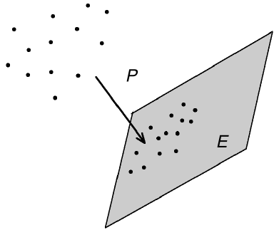
5.3 Application: Johnson-Lindenstrauss Lemma 117
5.3 Application: Johnson-Lindenstrauss Lemma
Suppose we have N data points in R
n
where n is very large. We would like to
reduce dimension of the data without sacrificing too much of its geometry. The
simplest form of dimension reduction is to project the data points onto a low-
dimensional subspace
E ⊂ R
n
, dim(E)
:
= m ≪ n,
see Figure 5.2 for illustration. How shall we choose the subspace E, and how
small its dimension m can be?
Figure 5.2 In Johnson-Lindenstrauss Lemma, the dimension of the data is
reduced by projection onto a random low-dimensional subspace.
Johnson-Lindenstrauss Lemma below states that the geometry of data is well
preserved if we choose E to be a random subspace of dimension
m ≍ log N.
We already came across the notion of a random subspace in Section 5.2.6; let us
recall it here. We say that E is a random m-dimensional subspace in R
n
uniformly
distributed in G
n,m
, i.e.
E ∼ Unif(G
n,m
),
if E is a random m-dimensional subspace of R
n
whose distribution is rotation
invariant, i.e.
P
E ∈ E
= P
U(E) ∈ E
for any fixed subset E ⊂ G
n,m
and n × n orthogonal matrix U.
Theorem 5.3.1 (Johnson-Lindenstrauss Lemma). Let X be a set of N points in
R
n
and ε > 0. Assume that
m ≥ (C/ε
2
) log N.

118 Concentration without independence
Consider a random m-dimensional subspace E in R
n
uniformly distributed in
G
n,m
. Denote the orthogonal projection onto E by P . Then, with probability at
least 1 − 2 exp(−cε
2
m), the scaled projection
Q
:
=
r
n
m
P
is an approximate isometry on X:
(1 − ε)∥x − y∥
2
≤ ∥Qx − Qy∥
2
≤ (1 + ε)∥x − y∥
2
for all x, y ∈ X. (5.10)
The proof of Johnson-Lindenstrauss Lemma will be based on concentration of
Lipschitz functions on the sphere, which we studied in Section 5.1. We use it to
first examine how the random projection P acts on a fixed vector x −y, and then
take union bound over all N
2
differences x − y.
Lemma 5.3.2 (Random projection). Let P be a projection in R
n
onto a random
m-dimensional subspace uniformly distributed in G
n,m
. Let z ∈ R
n
be a (fixed)
point and ε > 0. Then:
(a)
E ∥P z∥
2
2
1/2
=
r
m
n
∥z∥
2
.
(b) With probability at least 1 − 2 exp(−cε
2
m), we have
(1 − ε)
r
m
n
∥z∥
2
≤ ∥P z∥
2
≤ (1 + ε)
r
m
n
∥z∥
2
.
Proof Without loss of generality, we may assume that ∥z∥
2
= 1. (Why?) Next,
we consider an equivalent model: instead of a random projection P acting on a
fixed vector z, we consider a fixed projection P acting on a random vector z.
Specifically, the distribution of ∥P z∥
2
will not change if we let P be fixed and
z ∼ Unif(S
n−1
).
(Check this using rotation invariance!)
Using rotation invariance again, we may assume without loss of generality that
P is the coordinate projection onto the first m coordinates in R
n
. Thus
E ∥P z∥
2
2
= E
m
X
i=1
z
2
i
=
m
X
i=1
E z
2
i
= m E z
2
1
, (5.11)
since the coordinates z
i
of the random vector z ∼ Unif(S
n−1
) are identically
distributed. To compute E z
2
1
, note that
1 = ∥z∥
2
2
=
n
X
i=1
z
2
i
.
Taking expectations of both sides, we obtain
1 =
n
X
i=1
E z
2
i
= n E z
2
1
,

5.3 Application: Johnson-Lindenstrauss Lemma 119
which yields
E z
2
1
=
1
n
.
Putting this into (5.11), we get
E ∥P z∥
2
2
=
m
n
.
This proves the first part of the lemma.
The second part follows from concentration of Lipschitz functions on the sphere.
Indeed,
f(x)
:
= ∥P x∥
2
is a Lipschitz function on S
n−1
, and ∥f∥
Lip
= 1. (Check!) Then concentration
inequality (5.6) yields
P
(
∥P x∥
2
−
r
m
n
≥ t
)
≤ 2 exp(−cnt
2
).
(Here we also used Exercise 5.2.4 to replace E ∥x∥
2
by the (E ∥x∥
2
2
)
1/2
in the
concentration inequality.) Choosing t
:
= ε
p
m/n, we complete the proof of the
lemma.
Proof of Johnson-Lindenstrauss Lemma. Consider the difference set
X − X
:
= {x − y
:
x, y ∈ X}.
We would like to show that, with required probability, the inequality
(1 − ε)∥z∥
2
≤ ∥Qz∥
2
≤ (1 + ε)∥z∥
2
holds for all z ∈ X − X. Since Q =
p
n/m P , this is inequality is equivalent to
(1 − ε)
r
m
n
∥z∥
2
≤ ∥P z∥
2
≤ (1 + ε)
r
m
n
∥z∥
2
. (5.12)
For any fixed z, Lemma 5.3.2 states that (5.12) holds with probability at least
1 − 2 exp(−cε
2
m). It remains to take a union bound over z ∈ X − X. It follows
that inequality (5.12) holds simultaneously for all z ∈ X − X, with probability
at least
1 − |X − X| · 2 exp(−cε
2
m) ≥ 1 − N
2
· 2 exp(−cε
2
m).
If m ≥ (C/ε
2
) log N then this probability is at least 1 − 2 exp(−cε
2
m/2), as
claimed. Johnson-Lindenstrauss Lemma is proved.
A remarkable feature of Johnson-Lindenstrauss lemma is dimension reduction
map A is non-adaptive, it does not depend on the data. Note also that the ambient
dimension n of the data plays no role in this result.

120 Concentration without independence
Exercise 5.3.3 (Johnson-Lindenstrauss with sub-gaussian matrices). KKK Let
A be an m × n random matrix whose rows are independent, mean zero, sub-
gaussian isotropic random vectors in R
n
. Show that the conclusion of Johnson-
Lindenstrauss lemma holds for Q = (1/
√
m)A.
Exercise 5.3.4 (Optimality of Johnson-Lindenstrauss). KKK Give an exam-
ple of a set X of N points for which no scaled projection onto a subspace of
dimension m ≪ log N is an approximate isometry.
Hint: Set X be an orthogonal basis and show that the projected set defines a packing.
5.4 Matrix Bernstein’s inequality
In this section, we show how to generalize concentration inequalities for sums of
independent random variables
P
X
i
to sums of independent random matrices.
In this section, we prove a matrix version of Bernstein’s inequality (Theo-
rem 2.8.4), where the random variables X
i
are replaced by random matrices, and
the absolute value |·| is replaced by the operator norm ∥·∥. Remarkably, we will
not require independence of entries, rows, or columns within each random matrix
X
i
.
Theorem 5.4.1 (Matrix Bernstein’s inequality). Let X
1
, . . . , X
N
be independent,
mean zero, n ×n symmetric random matrices, such that ∥X
i
∥ ≤ K almost surely
for all i. Then, for every t ≥ 0, we have
P
N
X
i=1
X
i
≥ t
≤ 2n exp
−
t
2
/2
σ
2
+ Kt/3
.
Here σ
2
=
P
N
i=1
E X
2
i
is the norm of the matrix variance of the sum.
In particular, we can express this bound as the mixture of sub-gaussian and
sub-exponential tail, just like in the scalar Bernstein’s inequality:
P
N
X
i=1
X
i
≥ t
≤ 2n exp
− c · min
t
2
σ
2
,
t
K
.
The proof of matrix Bernstein’s inequality will be based on the following na¨ıve
idea. We try to repeat the classical argument based on moment generating func-
tions (see Section 2.8), replacing scalars by matrices at each occurrence. In most
of our argument this idea will work, except for one step that will be non-trivial to
generalize. Before we dive into this argument, let us develop some matrix calculus
which will allow us to treat matrices as scalars.
5.4.1 Matrix calculus
Throughout this section, we work with symmetric n × n matrices. As we know,
the operation of addition A + B generalizes painlessly from scalars to matrices.
We need to be more careful with multiplication, since it is not commutative for

5.4 Matrix Bernstein’s inequality 121
matrices: in general, AB ̸= BA. For this reason, matrix Bernstein’s inequality is
sometimes called non-commutative Bernstein’s inequality. Functions of matrices
are defined as follows.
Definition 5.4.2 (Functions of matrices). Consider a function f
:
R → R and
an n×n symmetric matrix X with eigenvalues λ
i
and corresponding eigenvectors
u
i
. Recall that X can be represented as a spectral decomposition
X =
n
X
i=1
λ
i
u
i
u
T
i
.
Then define
f(X)
:
=
n
X
i=1
f(λ
i
)u
i
u
T
i
.
In other words, to obtain the matrix f(X) from X, we do not change the eigen-
vectors and apply f to the eigenvalues.
In the following exercise, we check that the definition of function of matrices
agrees with the basic rules of matrix addition and multiplication.
Exercise 5.4.3 (Matrix polynomials and power series). KK
(a) Consider a polynomial
f(x) = a
0
+ a
1
x + ··· + a
p
x
p
.
Check that for a matrix X, we have
f(X) = a
0
I + a
1
X + ··· + a
p
X
p
.
In the right side, we use the standard rules for matrix addition and multi-
plication, so in particular X
p
= X ···X (p times) there.
(b) Consider a convergent power series expansion of f about x
0
:
f(x) =
∞
X
k=1
a
k
(x − x
0
)
k
.
Check that the series of matrix terms converges, and
f(X) =
∞
X
k=1
a
k
(X − x
0
I)
k
.
As an example, for each n × n symmetric matrix X we have
e
X
= I + X +
X
2
2!
+
X
3
3!
+ ···
Just like scalars, matrices can be compared to each other. To do this, we define
a partial order on the set of n × n symmetric matrices as follows.

122 Concentration without independence
Definition 5.4.4 (positive semidefinite order). Recall that
X ⪰ 0
if X is a symmetric positive semidefinite matrix. Equivalently, X ⪰ 0 if X is
symmetric and all eigenvalues of X satisfy λ
i
(X) ≥ 0. Next, we write
X ⪰ Y and Y ⪯ X
if X − Y ⪰ 0.
Note that ⪰ is a partial, as opposed to total, order, since there are matrices
for which neither X ⪰ Y nor Y ⪰ X hold. (Give an example!)
Exercise 5.4.5. KKK Prove the following properties.
(a) ∥X∥ ≤ t if and only if −tI ⪯ X ⪯ tI.
(b) Let f, g
:
R → R be two functions. If f(x) ≤ g(x) for all x ∈ R satisfying
|x| ≤ K, then f(X) ⪯ g(X) for all X satisfying ∥X∥ ≤ K.
(c) Let f
:
R → R be an increasing function and X, Y are commuting matrices.
Then X ⪯ Y implies f(X) ⪯ f(Y ).
(d) Give an example showing that property (c) may fail for non-commuting
matrices.
Hint: Find 2 × 2 matrices such that 0 ⪯ X ⪯ Y but X
2
̸⪯ Y
2
.
(e) In the following parts of the exercise, we develop weaker versions of prop-
erty (c) that hold for arbitrary, not necessarily commuting, matrices. First,
show that X ⪯ Y always implies tr f(X) ≤ tr f(Y ) for any increasing func-
tion f
:
R → R.
Hint: Using Courant-Fisher’s min-max principle (4.2), show that λ
i
(X) ≤ λ
i
(Y ) for all i.
(f) Show that 0 ⪯ X ⪯ Y implies X
−1
⪰ Y
−1
if X is invertible.
Hint: First consider the case where one of the matrices is the identity. Next, multiply the
inequality X ⪯ Y by Y
−1/2
on the left and on the right.
(g) Show that 0 ⪯ X ⪯ Y implies log X ⪯ log Y .
Hint: Check and use the identity log x =
R
∞
0
(
1
1+t
−
1
x+t
) dt and property (f).
5.4.2 Trace inequalities
So far, our attempts to extend scalar concepts for matrices have not met a con-
siderable resistance. But this does not always go so smoothly. We already saw
in Exercise 5.4.5 how the non-commutativity of the matrix product (AB ̸= BA)
may cause scalar properties to fail for matrices. Here is one more such situation:
the identity is e
x+y
= e
x
e
y
holds for scalars but fails for matrices.
Exercise 5.4.6. KKK Let X and Y be n × n symmetric matrices.
(a) Show that if the matrices commute, i.e. XY = Y X, then
e
X+Y
= e
X
e
Y
.
5.4 Matrix Bernstein’s inequality 123
(b) Find an example of matrices X and Y such that
e
X+Y
̸= e
X
e
Y
.
This is unfortunate for us, because we used the identity e
x+y
= e
x
e
y
in a crucial
way in our approach to concentration of sums of random variables. Indeed, this
identity allowed us to break the moment generating function E exp(λS) of the
sum into the product of exponentials, see (2.6).
Nevertheless, there exists useful substitutes for the missing identity e
X+Y
=
e
X
e
Y
. We state two of them here without proof; they belong to the rich family
of trace inequalities.
Theorem 5.4.7 (Golden-Thompson inequality). For any n × n symmetric ma-
trices A and B, we have
tr(e
A+B
) ≤ tr(e
A
e
B
).
Unfortunately, Goldon-Thpmpson inequality does not hold for three or more
matrices: in general, the inequality tr(e
A+B+C
) ≤ tr(e
A
e
B
e
C
) may fail.
Theorem 5.4.8 (Lieb’s inequality). Let H be an n×n symmetric matrix. Define
the function on matrices
f(X)
:
= tr exp(H + log X).
Then f is concave on the space on positive definite n × n symmetric matrices.
13
Note that in the scalar case where n = 1, the function f is linear and Lieb’s
inequality holds trivially.
A proof of matrix Bernstein’s inequality can be based on either Golden-Thompson
or Lieb’s inequalities. We use Lieb’s inequality, which we will now restate for ran-
dom matrices. If X is a random matrix, then Lieb’s and Jensen’s inequalities
imply that
E f(X) ≤ f(E X).
(Why does Jensen’s inequality hold for random matrices?) Applying this with
X = e
Z
, we obtain the following.
Lemma 5.4.9 (Lieb’s inequality for random matrices). Let H be a fixed n × n
symmetric matrix and Z be a random n × n symmetric matrix. Then
E tr exp(H + Z) ≤ tr exp(H + log E e
Z
).
5.4.3 Proof of matrix Bernstein’s inequality
We are now ready to prove matrix Bernstein’s inequality, Theorem 5.4.1, using
Lieb’s inequality.
13
Concavity means that the inequality f (λX + (1 − λ)Y ) ≥ λf (X) + (1 −λ)f (Y ) holds for matrices X
and Y , and for λ ∈ [0, 1].
124 Concentration without independence
Step 1: Reduction to MGF. To bound the norm of the sum
S
:
=
N
X
i=1
X
i
,
we need to control the largest and smallest eigenvalues of S. We can do this
separately. To put this formally, consider the largest eigenvalue
λ
max
(S)
:
= max
i
λ
i
(S)
and note that
∥S∥ = max
i
|λ
i
(S)| = max
λ
max
(S), λ
max
(−S)
. (5.13)
To bound λ
max
(S), we proceed with the method based on computing the mo-
ment generating function as we did in the scalar case, e.g. in Section 2.2. To this
end, fix λ ≥ 0 and use Markov’s inequality to obtain
P
λ
max
(S) ≥ t
= P
n
e
λ·λ
max
(S)
≥ e
λt
o
≤ e
−λt
E e
λ·λ
max
(S)
. (5.14)
Since by Definition 5.4.2 the eigenvalues of e
λS
are e
λ·λ
i
(S)
, we have
E
:
= E e
λ·λ
max
(S)
= E λ
max
(e
λS
).
Since the eigenvalues of e
λS
are all positive, the maximal eigenvalue of e
λS
is
bounded by the sum of all eigenvalues, the trace of e
λS
, which leads to
E ≤ E tr e
λS
.
Step 2: Application of Lieb’s inequality. To prepare for an application of
Lieb’s inequality (Lemma 5.4.9), let us separate the last term from the sum S:
E ≤ E tr exp
N−1
X
i=1
λX
i
+ λX
N
.
Condition on (X
i
)
N−1
i=1
and apply Lemma 5.4.9 for the fixed matrix H
:
=
P
N−1
i=1
λX
i
and the random matrix Z
:
= λX
N
. We obtain
E ≤ E tr exp
N−1
X
i=1
λX
i
+ log E e
λX
N
.
(To be more specific here, we first apply Lemma 5.4.9 for the conditional expecta-
tion, and then take expectation of both sides using the law of total expectation.)
We continue in a similar way: separate the next term λX
N−1
from the sum
P
N−1
i=1
λX
i
and apply Lemma 5.4.9 again for Z = λX
N−1
. Repeating N times, we
obtain
E ≤ tr exp
N
X
i=1
log E e
λX
i
. (5.15)

5.4 Matrix Bernstein’s inequality 125
Step 3: MGF of the individual terms. It remains to bound the matrix-
valued moment generating function E e
λX
i
for each term X
i
. This is a standard
task, and the argument will be similar to the scalar case.
Lemma 5.4.10 (Moment generating function). Let X be an n × n symmetric
mean zero random matrix such that ∥X∥ ≤ K almost surely. Then
E exp(λX) ⪯ exp
g(λ) E X
2
where g(λ) =
λ
2
/2
1 − |λ|K/3
,
provided that |λ| < 3/K.
Proof First, note that we can bound the (scalar) exponential function by the
first few terms of its Taylor’s expansion as follows:
e
z
≤ 1 + z +
1
1 − |z|/3
·
z
2
2
, if |z| < 3.
(To get this inequality, write e
z
= 1 + z + z
2
·
P
∞
p=2
z
p−2
/p! and use the bound
p! ≥ 2 · 3
p−2
.) Next, apply this inequality for z = λx. If |x| ≤ K and |λ| < 3/K
then we obtain
e
λx
≤ 1 + λx + g(λ)x
2
,
where g(λ) is the function in the statement of the lemma.
Finally, we can transfer this inequality from scalars to matrices using part (b)
of Exercise 5.4.5. We obtain that if ∥X∥ ≤ K and |λ| < 3/K, then
e
λX
⪯ I + λX + g(λ)X
2
.
Take expectation of both sides and use the assumption that E X = 0 to obtain
E e
λX
⪯ I + g(λ) E X
2
.
To bound the right hand side, we may use the inequality 1 + z ≤ e
z
which holds
for all scalars z. Thus the inequality I + Z ⪯ e
Z
holds for all matrices Z, and in
particular for Z = g(λ) E X
2
. (Here we again refer to part (b) of Exercise 5.4.5.)
This yields the conclusion of the lemma.
Step 4: Completion of the proof. Let us return to bounding the quantity
in (5.15). Using Lemma 5.4.10, we obtain
E ≤ tr exp
N
X
i=1
log E e
λX
i
≤ tr exp
g(λ)Z
, where Z
:
=
N
X
i=1
E X
2
i
.
(Here we used Exercise 5.4.5 again: part (g) to take logarithms on both sides,
and then part (e) to take traces of the exponential of both sides.)
Since the trace of exp
g(λ)Z
is a sum of n positive eigenvalues, it is bounded
by n times the maximum eigenvalue, so
E ≤ n · λ
max
exp[g(λ)Z]
= n · exp
g(λ)λ
max
(Z)
(why?)
= n · exp
g(λ)∥Z∥
(since Z ⪰ 0)
= n · exp
g(λ)σ
2
(by definition of σ in the theorem).

126 Concentration without independence
Plugging this bound for E = E e
λ·λ
max
(S)
into (5.14), we obtain
P
λ
max
(S) ≥ t
≤ n · exp
−λt + g(λ)σ
2
.
We obtained a bound that holds for any λ > 0 such that |λ| < 3/K, so we can
minimize it in λ. Better yet, instead of computing the exact minimum (which
might be a little too ugly), we can choose the following value: λ = t/(σ
2
+ Kt/3).
Substituting it into the bound above and simplifying yields
P
λ
max
(S) ≥ t
≤ n · exp
−
t
2
/2
σ
2
+ Kt/3
.
Repeating the argument for −S and combining the two bounds via (5.13), we
complete the proof of Theorem 5.4.1. (Do this!)
5.4.4 Matrix Khintchine’s inequality
Matrix Bernstein’s inequality gives a good tail bound on ∥
P
N
i=1
X
i
∥, and this in
particular implies a non-trivial bound on the expectation:
Exercise 5.4.11 (Matrix Bernstein’s inequality: expectation). KKK Let X
1
, . . . , X
N
be independent, mean zero, n ×n symmetric random matrices, such that ∥X
i
∥ ≤
K almost surely for all i. Deduce from Bernstein’s inequality that
E
N
X
i=1
X
i
≲
N
X
i=1
E X
2
i
1/2
p
1 + log n + K(1 + log n).
Hint: Check that matrix Bernstein’s inequality implies that
P
N
i=1
X
i
≲
P
N
i=1
E X
2
i
1/2
√
log n + u+
K(log n + u) with probability at least 1 − 2e
−u
. Then use the integral identity from Lemma 1.2.1.
Note that in the scalar case where n = 1, a bound on the expectation is trivial.
Indeed, in this case we have
E
N
X
i=1
X
i
≤
E
N
X
i=1
X
i
2
1/2
=
N
X
i=1
E X
2
i
1/2
.
where we used that the variance of a sum of independent random variables equals
the sum of variances.
The techniques we developed in the proof of matrix Bernstein’s inequality can
be used to give matrix versions of other classical concentration inequalities. In
the next two exercises, you will prove matrix versions of Hoeffding’s inequality
(Theorem 2.2.2) and Khintchine’s inequality (Exercise 2.6.6).
Exercise 5.4.12 (Matrix Hoeffding’s inequality). KKK Let ε
1
, . . . , ε
n
be inde-
pendent symmetric Bernoulli random variables and let A
1
, . . . , A
N
be symmetric
n × n matrices (deterministic). Prove that, for any t ≥ 0, we have
P
N
X
i=1
ε
i
A
i
≥ t
≤ 2n exp(−t
2
/2σ
2
),

5.4 Matrix Bernstein’s inequality 127
where σ
2
=
P
N
i=1
A
2
i
.
Hint: Proceed like in the proof of Theorem 5.4.1. Instead of Lemma 5.4.10, check that E exp(λε
i
A
i
) ⪯
exp(λ
2
A
2
i
/2) just like in the proof of Hoeffding’s inequality, Theorem 2.2.2.
From this, one can deduce a matrix version of Khintchine’s inequality:
Exercise 5.4.13 (Matrix Khintchine’s inequality). KKK Let ε
1
, . . . , ε
N
be in-
dependent symmetric Bernoulli random variables and let A
1
, . . . , A
N
be symmet-
ric n × n matrices (deterministic).
(a) Prove that
E
N
X
i=1
ε
i
A
i
≤ C
p
1 + log n
N
X
i=1
A
2
i
1/2
.
(b) More generally, prove that for every p ∈ [1, ∞) we have
E
N
X
i=1
ε
i
A
i
p
1/p
≤ C
p
p + log n
N
X
i=1
A
2
i
1/2
.
The price of going from scalar to matrices is the pre-factor n in the probability
bound in Theorem 5.4.1. This is a small price, considering that this factor becomes
logarithmic in dimension n in the expectation bound of Exercises 5.4.11–5.4.13.
The following example demonstrates that the logarithmic factor is needed in
general.
Exercise 5.4.14 (Sharpness of matrix Bernstein’s inequality). KKK Let X
be an n × n random matrix that takes values e
k
e
T
k
, k = 1, . . . , n, with probabil-
ity 1/n each. (Here (e
k
) denotes the standard basis in R
n
.) Let X
1
, . . . , X
N
be
independent copies of X. Consider the sum
S
:
=
N
X
i=1
X
i
,
which is a diagonal matrix.
(a) Show that the entry S
ii
has the same distribution as the number of balls
in i-th bin when N balls are thrown into n bins independently.
(b) Relating this to the classical coupon collector’s problem, show that if N ≍ n
then
14
E ∥S∥ ≍
log n
log log n
.
Deduce that the bound in Exercise 5.4.11 would fail if the logarithmic
factors were removed from it.
The following exercise extends matrix Bernstein’s inequality by dropping both
the symmetry and square assumption on the matrices X
i
.
14
Here we write a
n
≍ b
n
if there exist constants c, C > 0 such that ca
n
< b
n
≤ Ca
n
for all n.

128 Concentration without independence
Exercise 5.4.15 (Matrix Bernstein’s inequality for rectangular matrices). KKK
Let X
1
, . . . , X
N
be independent, mean zero, m × n random matrices, such that
∥X
i
∥ ≤ K almost surely for all i. Prove that for t ≥ 0, we have
P
N
X
i=1
X
i
≥ t
≤ 2(m + n) exp
−
t
2
/2
σ
2
+ Kt/3
,
where
σ
2
= max
N
X
i=1
E X
T
i
X
i
,
N
X
i=1
E X
i
X
T
i
.
Hint: Apply matrix Bernstein’s inequality (Theorem 5.4.1) for the sum of (m + n) ×(m + n) symmetric
matrices
h
0 X
T
i
X
i
0
i
.
5.5 Application: community detection in sparse networks
In Section 4.5, we analyzed a basic method for community detection in networks
– the spectral clustering algorithm. We examined the performance of spectral
clustering for the stochastic block model G(n, p, q) with two communities, and
we found how the communities can be identified with high accuracy and high
probability (Theorem 4.5.6).
We now re-examine the performance of spectral clustering using matrix Bern-
stein’s inequality. In the following two exercises, we find that spectral cluster-
ing actually works for much sparser networks than we knew before from Theo-
rem 4.5.6.
Just like in Section 4.5, we denote by A the adjacency matrix of a random
graph from G(n, p, q), and we express A as
A = D + R
where D = E A is a deterministic matrix (“signal”) and R is random (“noise”).
As we know, the success of spectral clustering method hinges on the fact that the
noise ∥R∥ is small with high probability (recall (4.18)). In the following exercise,
you will use Matrix Bernstein’s inequality to derive a better bound on ∥R∥.
Exercise 5.5.1 (Controlling the noise). KKK
(a) Represent the adjacency matrix A as a sum of independent random matri-
ces
A =
X
1≤i≤j≤n
Z
ij
.
Make it so that each Z
ij
encode the contribution of an edge between vertices
i and j. Thus, the only non-zero entries of Z
ij
should be (ij) and (ji), and
they should be the same as in A.
(b) Apply matrix Bernstein’s inequality to find that
E ∥R∥ ≲
p
d log n + log n,

5.6 Application: covariance estimation for general distributions 129
where d =
1
2
(p + q)n is the expected average degree of the graph.
Exercise 5.5.2 (Spectral clustering for sparse networks). KKK Use the bound
from Exercise 5.5.1 to give better guarantees for the performance of spectral
clustering than we had in Section 4.5. In particular, argue that spectral clustering
works for sparse networks, as long as the average expected degrees satisfy
d ≫ log n.
5.6 Application: covariance estimation for general distributions
In Section 4.7, we saw how the covariance matrix of a sub-gaussian distribution
in R
n
can be accurately estimated using a sample of size O(n). In this section,
we remove the sub-gaussian requirement, and thus make covariance estimation
possible for very general, in particular discrete, distributions. The price we pay
is very small – just a logarithmic oversampling factor.
Like in Section 4.7, we estimate the the second moment matrix Σ = E XX
T
by
its sample version
Σ
m
=
1
m
m
X
i=1
X
i
X
T
i
.
Recall that if X has zero mean, then Σ is the covariance matrix of X and Σ
m
is
the sample covariance matrix of X.
Theorem 5.6.1 (General covariance estimation). Let X be a random vector in
R
n
, n ≥ 2. Assume that for some K ≥ 1,
∥X∥
2
≤ K (E ∥X∥
2
2
)
1/2
almost surely. (5.16)
Then, for every positive integer m, we have
E ∥Σ
m
− Σ∥ ≤ C
r
K
2
n log n
m
+
K
2
n log n
m
∥Σ∥.
Proof Before we start proving the bound, let us pause to note that E ∥X∥
2
2
=
tr(Σ). (Check this like in the proof of Lemma 3.2.4.) So the assumption (5.16)
becomes
∥X∥
2
2
≤ K
2
tr(Σ) almost surely. (5.17)
Apply the expectation version of matrix Bernstein’s inequality (Exercise 5.4.11)
for the sum of i.i.d. mean zero random matrices X
i
X
T
i
− Σ and get
15
E ∥Σ
m
− Σ∥ =
1
m
E
m
X
i=1
(X
i
X
T
i
− Σ)
≲
1
m
σ
p
log n + M log n
(5.18)
15
As usual, the notation a ≲ b hides absolute constant factors, i.e. it means that a ≤ Cb where C is an
absolute constant.

130 Concentration without independence
where
σ
2
=
m
X
i=1
E(X
i
X
T
i
− Σ)
2
= m
E(XX
T
− Σ)
2
and M is any number chosen so that
∥XX
T
− Σ∥ ≤ M almost surely.
To complete the proof, it remains to bound σ
2
and M.
Let us start with σ
2
. Expanding the square, we find that
16
E(XX
T
− Σ)
2
= E(XX
T
)
2
− Σ
2
⪯ E(XX
T
)
2
. (5.19)
Further, the assumption (5.17) gives
(XX
T
)
2
= ∥X∥
2
XX
T
⪯ K
2
tr(Σ)XX
T
.
Taking expectation and recalling that E XX
T
= Σ, we obtain
E(XX
T
)
2
⪯ K
2
tr(Σ)Σ.
Substituting this bound into (5.19), we obtain a good bound on σ, namely
σ
2
≤ K
2
m tr(Σ)∥Σ∥.
Bounding M is simple: indeed,
∥XX
T
− Σ∥ ≤ ∥X∥
2
2
+ ∥Σ∥ (by triangle inequality)
≤ K
2
tr(Σ) + ∥Σ∥ (by assumption (5.17))
≤ 2K
2
tr(Σ) =
:
M (since ∥Σ∥ ≤ tr(Σ) and K ≥ 1).
Substituting our bounds for σ and M into (5.18), we get
E ∥Σ
m
− Σ∥ ≤
1
m
q
K
2
m tr(Σ)∥Σ∥ ·
p
log n + 2K
2
tr(Σ) · log n
.
To complete the proof, use the inequality tr(Σ) ≤ n∥Σ∥ and simplify the bound.
Remark 5.6.2 (Sample complexity). Theorem 5.6.1 implies that for any ε ∈
(0, 1), we are guaranteed to have covariance estimation with a good relative error,
E ∥Σ
m
− Σ∥ ≤ ε∥Σ∥, (5.20)
if we take a sample of size
m ≍ ε
−2
n log n.
Compare this with the sample complexity m ≍ ε
−2
n for sub-gaussian distribu-
tions (recall Remark 4.7.2). We see that the price of dropping the sub-gaussian
requirement turned out to be very small – it is just a logarithmic oversampling
factor.
16
Recall Definition 5.4.4 of the positive semidefinite order ⪯ used here.

5.6 Application: covariance estimation for general distributions 131
Remark 5.6.3 (Lower-dimensional distributions). At the end of the proof of
Theorem 5.6.1, we used a crude bound tr(Σ) ≤ n∥Σ∥. But we may chose not to
do that, and instead get a bound in terms of the intrinsic dimension
r =
tr(Σ)
∥Σ∥
,
namely
E ∥Σ
m
− Σ∥ ≤ C
r
K
2
r log n
m
+
K
2
r log n
m
∥Σ∥.
In particular, this stronger bound implies that a sample of size
m ≍ ε
−2
r log n
is sufficient to estimate the covariance matrix as in (5.20). Note that we always
have r ≤ n (why?), so the new bound is always as good as the one in Theo-
rem 5.6.1. But for approximately low dimensional distributions – those that tend
to concentrate near low-dimensional subspaces – we may have r ≪ n, and in
this case estimate covariance using a much smaller sample. We will return to this
discussion in Section 7.6 where we introduce the notions of stable dimension and
stable rank.
Exercise 5.6.4 (Tail bound). KK Our argument also implies the following
high-probability guarantee. Check that for any u ≥ 0, we have
∥Σ
m
− Σ∥ ≤ C
r
K
2
r(log n + u)
m
+
K
2
r(log n + u)
m
∥Σ∥
with probability at least 1 − 2e
−u
. Here r = tr(Σ)/∥Σ∥ ≤ n as before.
Exercise 5.6.5 (Necessity of boundedness assumption). KKK Show that if the
boundedness assumption (5.16) is removed from Theorem 5.6.1, the conclusion
may fail in general.
Exercise 5.6.6 (Sampling from frames). KK Consider an equal-norm tight
frame
17
(u
i
)
N
i=1
in R
n
. State and prove a result that shows that a random sample
of
m ≳ n log n
elements of (u
i
) forms a frame with good frame bounds (as close to tight as one
wants). The quality of the result should not depend on the frame size N.
Exercise 5.6.7 (Necessity of logarithmic oversampling). KK Show that in gen-
eral, logarithmic oversampling is necessary for covariance estimation. More pre-
cisely, give an example of a distribution in R
n
for which the bound (5.20) must
fail for every ε < 1 unless m ≳ n log n.
Hint: Think about the coordinate distribution from Section 3.3.4; argue like in Exercise 5.4.14.
17
The concept of frames was introduced in Section 3.3.4. By equal-norm frame we mean that
∥u
i
∥
2
= ∥u
j
∥
2
for all i and j.
132 Concentration without independence
Exercise 5.6.8 (Random matrices with general independent rows). KKK Prove
a version of Theorem 4.6.1 which holds for random matrices with arbitrary, not
necessarily sub-gaussian distributions of rows.
Let A be an m × n matrix whose rows A
i
are independent isotropic random
vectors in R
n
. Assume that for some K ≥ 0,
∥A
i
∥
2
≤ K
√
n almost surely for every i. (5.21)
Prove that, for every t ≥ 1, one has
√
m − Kt
p
n log n ≤ s
n
(A) ≤ s
1
(A) ≤
√
m + Kt
p
n log n (5.22)
with probability at least 1 − 2n
−ct
2
.
Hint: Just like in the proof of Theorem 4.6.1, derive the conclusion from a bound on
1
m
A
T
A − I
n
=
1
m
P
m
i=1
A
i
A
T
i
− I
n
. Use the result of Exercise 5.6.4.
5.7 Notes
There are several introductory texts about concentration, such as [11, Chapter 3],
[150, 130, 129, 30] and an elementary tutorial [13].
The approach to concentration via isoperimetric inequalities that we presented
in Section 5.1 was fist discovered by P. L´evy, to whom Theorems 5.1.5 and 5.1.4
are due (see [91]).
When V. Milman realized the power and generality of L´evy’s approach in 1970-
s, this led to far-reaching extensions of the concentration of measure principle,
some of which we surveyed in Section 5.2. To keep this book concise, we left out
a lot of important approaches to concentration, including bounded differences
inequality, martingale, semigroup and transportation methods, Poincare inequal-
ity, log-Sobolev inequality, hypercontractivity, Stein’s method and Talagrand’s
concentration inequalities see [212, 129, 30]. Most of the material we covered in
Sections 5.1 and 5.2 can be found in [11, Chapter 3], [150, 129].
The Gaussian isoperimetric inequality (Theorem 5.2.1) was first proved by
V. N. Sudakov and B. S. Cirelson (Tsirelson) and independently by C. Borell [28].
There are several other proofs of Gaussian isoperimetric inequality, see [24, 12, 16].
There is also an elementary derivation of Gaussian concentration (Theorem 5.2.2)
from Gaussian interpolation instead of isoperimetry, see [167].
Concentration on the Hamming cube (Theorem 5.2.5) is a consequence of
Harper’s theorem, which is an isoperimetric inequality for the Hamming cube
[98], see [25]. Concentration on the symmetric group (Theorem 5.2.6) is due to
B. Maurey [139]. Both Theorems 5.2.5 and 5.2.6 can be also proved using mar-
tingale methods, see [150, Chapter 7].
The proof of concentration on Riemannian manifolds with positive curvature
(inequality [129, Section 2.3]) can be found e.g. in [129, Proposition 2.17]. Many
interesting special cases follow from this general result, including Theorem 5.2.7
for the special orthogonal group [150, Section 6.5.1] and, consequently, Theo-
rem 5.2.9 for the Grassmannian [150, Section 6.7.2]. A construction of Haar mea-
sure we mentioned in Remark 5.2.8 can be found e.g. in [150, Chapter 1] and
5.7 Notes 133
[76, Chapter 2]; the survey [147] discusses numerically stable ways to generate
random unitary matrices.
Concentration on the continuous cube (Theorem 5.2.10) can be found in [129,
Proposition 2.8], and concentration on the Euclidean ball (Theorem 5.2.13), in
[129, Proposition 2.9]. Theorem 5.2.15 on concentration for exponential densities
is borrowed from [129, Proposition 2.18]. The proof of Talagrand’s concentration
inequality (Theorem 5.2.16) originally can be found in [198, Theorem 6.6], [129,
Corollary 4.10].
The original formulation of Johnson-Lindenstrauss Lemma is from [110]. For
various versions of this lemma, related results, applications, and bibliographic
notes, see [138, Section 15.2]. The condition m ≳ ε
−2
log N is known to be optimal
[124].
The approach to matrix concentration inequalities we follow in Section 5.4 orig-
inates in the work of R. Ahlswede and A. Winter [4]. A short proof of Golden-
Thompson inequality (Theorem 5.4.7), a result on which Ahlswede-Winter’s ap-
proach rests, can be found e.g. in [21, Theorem 9.3.7] and [221]. While the work of
R. Ahlswede and A. Winter was motivated by problems of quantum information
theory, the usefulness of their approach was gradually understood in other areas
as well; the early work includes [227, 220, 92, 159].
The original argument of R. Ahlswede and A. Winter yields a version of matrix
Bernstein’s inequality that is somewhat weaker than Theorem 5.4.1, namely with
P
N
i=1
∥E X
2
i
∥ instead of σ. This quantity was later tightened by R. Oliveira [160]
by a modification of Ahlswede-Winter’s method and independently by J. Tropp [206]
using Lieb’s inequality (Theorem 5.4.8) instead of Golden-Thompson’s. In this
book, we mainly follow J. Tropp’s proof of Theorem 5.4.1. The book [207] presents
a self-contained proof of Lieb’s inequality (Theorem 5.4.8), matrix Hoeffding’s in-
equality from Exercise 5.4.12, matrix Chernoff inequality, and much more. Due to
J. Tropp’s contributions, now there exist matrix analogs of almost all of the clas-
sical scalar concentration results [207]. The survey [165] discusses several other
useful trace inequalities and outlines proofs of Golden-Thompson inequality (in
Section 3) and Lieb’s inequality (embedded in the proof of Proposition 7). The
book [78] also contains a detailed exposition of matrix Bernstein’s inequality and
Instead of using matrix Bernstein’s inequality, one can deduce the result of
Exercise 5.4.11 from Gaussian integration by parts and a trace inequality [209].
Matrix Khintchine inequality from Exercise 5.4.13 can alternatively be deduced
from non-commutative Khintchine’s inequality due to F. Lust-Piquard [134]; see
also [135, 40, 41, 172]. This derivation was first observed and used by M. Rudelson
[175] who proved a version of Exercise 5.4.13.
For the problem of community detection in networks we discussed in Sec-
tion 5.5, see the notes at the end of Chapter 4. The approach to concentration
of random graphs using matrix Bernstein’s inequality we outlined in Section 5.5
was first proposed by R. Oliveira [160].
In Section 5.6 we discussed covariance estimation for general high-dimensional
distributions following [222]. An alternative and earlier approach to covariance
134 Concentration without independence
estimation, which gives similar results, relies on matrix Khintchine’s inequalities
(known as non-commutative Khintchine inequalities); it was developed earlier
by M. Rudelson [175]. For more references on covariance estimation problem,
see the notes at the end of Chapter 4. The result of Exercise 5.6.8 is from [222,
Section 5.4.2].

6
Quadratic forms, symmetrization and
contraction
In this chapter, we introduce a number of basic tools of high-dimensional proba-
bility: decoupling in Section 6.1, concentration of quadratic forms (the Hanson-
Wright inequality) in Section 6.2, symmetrization in Section 6.4 and contraction
in Section 6.7.
We illustrate these tools in a number of applications. In Section 6.3, we use
the Hanson-Wright inequality to establish concentration for anisotropic random
vectors (thus extending Theorem 3.1.1) and for the distances between random
vectors and subspaces. In Section 6.5, we combine matrix Bernstein’s inequality
with symmetrization arguments to analyze the operator norm of a random matrix;
we show that it is almost equivalent to the largest Euclidean norm of the rows and
columns. We use this result in Section 6.6 for the problem of matrix completion,
where one is shown a few randomly chosen entries of a given matrix and is asked
to fill in the missing entries.
6.1 Decoupling
In the beginning of this book, we thoroughly studied independent random vari-
ables of the type
n
X
i=1
a
i
X
i
(6.1)
where X
1
, . . . , X
n
are independent random variables and a
i
are fixed coefficients.
In this section, we study quadratic forms of the type
n
X
i,j=1
a
ij
X
i
X
j
= X
T
AX = ⟨X, AX⟩ (6.2)
where A = (a
ij
) is an n × n matrix of coefficients, and X = (X
1
, . . . , X
n
) is a
random vector with independent coordinates. Such a quadratic form is called a
chaos in probability theory.
Computing the expectation of a chaos is easy. For simplicity, let us assume that
X
i
have zero means and unit variances. Then
E X
T
AX =
n
X
i,j=1
a
ij
E X
i
X
j
=
n
X
i=1
a
ii
= tr A.
135

136 Quadratic forms, symmetrization and contraction
It is harder to establish a concentration of a chaos. The main difficulty is that
the terms of the sum in (6.2) are not independent. This difficulty can be overcome
by the decoupling technique, which we will study now.
The purpose of decoupling is to replace the quadratic form (6.2) with the
bilinear form
n
X
i,j=1
a
ij
X
i
X
′
j
= X
T
AX
′
=
X, AX
′
,
where X
′
= (X
′
1
, . . . , X
′
n
) is a random vector which is independent of X yet has
the same distribution as X. Such X
′
is called an independent copy of X. The
point here is that the bilinear form is easier to analyze than the quadratic form,
since it is linear in X. Indeed, if we condition on X
′
we may treat the bilinear
form as a sum of independent random variables
n
X
i=1
n
X
j=1
a
ij
X
′
j
X
i
=
n
X
i=1
c
i
X
i
with fixed coefficients c
i
, much like we treated the sums (6.1) before.
Theorem 6.1.1 (Decoupling). Let A be an n ×n, diagonal-free matrix (i.e. the
diagonal entries of A equal zero). Let X = (X
1
, . . . , X
n
) be a random vector with
independent mean zero coordinates X
i
. Then, for every convex function F
:
R →
R, one has
E F (X
T
AX) ≤ E F (4X
T
AX
′
) (6.3)
where X
′
is an independent copy of X.
The proof will be based on the following observation.
Lemma 6.1.2. Let Y and Z be independent random variables such that E Z = 0.
Then, for every convex function F , one has
E F (Y ) ≤ E F (Y + Z).
Proof This is a simple consequence of Jensen’s inequality. First let us fix an
arbitrary y ∈ R and use E Z = 0 to get
F (y) = F (y + E Z) = F (E[y + Z]) ≤ E F (y + Z).
Now choose y = Y and take expectations of both sides to complete the proof. (To
check if you understood this argument, find where the independence of Y and Z
was used!)
Proof of Decoupling Theorem 6.1.1 Here is what our proof will look like in a
nutshell. First, we replace the chaos X
T
AX =
P
i,j
a
ij
X
i
X
j
by the “partial chaos”
X
(i,j)∈I×I
c
a
ij
X
i
X
j
where the subset of indices I ⊂ {1, . . . , n} will be chosen by random sampling.

6.1 Decoupling 137
The advantage of partial chaos is that the summation is done over disjoint sets
for i and j. Thus one can automatically replace X
j
by X
′
j
without changing the
distribution. Finally, we complete the partial chaos to the full sum X
T
AX
′
=
P
i,j
a
ij
X
i
X
′
j
using Lemma 6.1.2.
Now we pass to a detailed proof. To randomly select a subset of indices I, let
us consider selectors δ
1
, . . . , δ
n
∈ {0, 1}, which are independent Bernoulli random
variables with P{δ
i
= 0} = P{δ
i
= 1} = 1/2. Define
I
:
= {i
:
δ
i
= 1}.
Condition on X. Since by assumption a
ii
= 0 and
E δ
i
(1 − δ
j
) =
1
2
·
1
2
=
1
4
for all i ̸= j,
we may express the chaos as
X
T
AX =
X
i̸=j
a
ij
X
i
X
j
= 4 E
δ
X
i̸=j
δ
i
(1 − δ
j
)a
ij
X
i
X
j
= 4 E
I
X
(i,j)∈I×I
c
a
ij
X
i
X
j
.
(The subscripts δ and I are meant to remind us about the sources of randomness
used in taking these conditional expectations. Since we fixed X, the conditional
expectations are over the random selectors δ = (δ
1
, . . . , δ
n
), or equivalently, over
the random set of indices I. We will continue to use similar notation later.)
Apply the function F to both sides and take expectation over X. Using Jensen’s
inequality and Fubini theorem, we obtain
E
X
F (X
T
AX) ≤ E
I
E
X
F
4
X
(i,j)∈I×I
c
a
ij
X
i
X
j
.
It follows that there exists a realization of a random subset I such that
E
X
F (X
T
AX) ≤ E
X
F
4
X
(i,j)∈I×I
c
a
ij
X
i
X
j
.
Fix such realization of I until the end of the proof (and drop the subscripts
X in the expectation for convenience.) Since the random variables (X
i
)
i∈I
are
independent from (X
j
)
j∈I
c
, the distribution of the sum in the right side will not
change if we replace X
j
by X
′
j
. So we get
E F (X
T
AX) ≤ E F
4
X
(i,j)∈I×I
c
a
ij
X
i
X
′
j
.
It remains to complete the sum in the right side to the sum over all pairs of
indices. In other words, we want to show that
E F
4
X
(i,j)∈I×I
c
a
ij
X
i
X
′
j
≤ E F
4
X
(i,j)∈[n]×[n]
a
ij
X
i
X
′
j
, (6.4)
where we use the notation [n] = {1, . . . , n}. To do this, we decompose the sum

138 Quadratic forms, symmetrization and contraction
in the right side as
X
(i,j)∈[n]×[n]
a
ij
X
i
X
′
j
= Y + Z
1
+ Z
2
where
Y =
X
(i,j)∈I×I
c
a
ij
X
i
X
′
j
, Z
1
=
X
(i,j)∈I×I
a
ij
X
i
X
′
j
, Z
2
=
X
(i,j)∈I
c
×[n]
a
ij
X
i
X
′
j
.
Condition on all random variables except (X
′
j
)
j∈I
and (X
i
)
i∈I
c
. This fixes Y , while
Z
1
and Z
2
are random variables with zero conditional expectations (check!). Use
Lemma 6.1.2 to conclude that the conditional expectation, which we denote E
′
,
satisfies
F (4Y ) ≤ E
′
F (4Y + 4Z
1
+ 4Z
2
).
Finally, taking expectation of both sides over all other random variables, we
conclude that
E F (4Y ) ≤ E F (4Y + 4Z
1
+ 4Z
2
).
This proves (6.4) and finishes the argument.
Remark 6.1.3. We actually proved a slightly stronger version of decoupling
inequality, in which A needs not be diagonal-free. Thus, for any square matrix
A = (a
ij
) we showed that
E F
X
i,j
:
i̸=j
a
ij
X
i
X
j
≤ E F
4
X
i,j
a
ij
X
i
X
′
j
Exercise 6.1.4 (Decoupling in Hilbert spaces). K Prove the following gener-
alization of Theorem 6.1.1. Let A = (a
ij
) be an n × n matrix. Let X
1
, . . . , X
n
be independent, mean zero random vectors in some Hilbert space. Show that for
every convex function F
:
R → R, one has
E F
X
i,j
:
i̸=j
a
ij
X
i
, X
j
≤ E F
4
X
i,j
a
ij
D
X
i
, X
′
j
E
,
where (X
′
i
) is an independent copy of (X
i
).
Exercise 6.1.5 (Decoupling in normed spaces). KK Prove the following al-
ternative generalization of Theorem 6.1.1. Let (u
ij
)
n
i,j=1
be fixed vectors in some
normed space. Let X
1
, . . . , X
n
be independent, mean zero random variables. Show
that, for every convex and increasing function F , one has
E F
X
i,j
:
i̸=j
X
i
X
j
u
ij
≤ E F
4
X
i,j
X
i
X
′
j
u
ij
.
where (X
′
i
) is an independent copy of (X
i
).

6.2 Hanson-Wright Inequality 139
6.2 Hanson-Wright Inequality
We now prove a general concentration inequality for a chaos. It can be viewed as
a chaos version of Bernstein’s inequalty.
Theorem 6.2.1 (Hanson-Wright inequality). Let X = (X
1
, . . . , X
n
) ∈ R
n
be a
random vector with independent, mean zero, sub-gaussian coordinates. Let A be
an n × n matrix. Then, for every t ≥ 0, we have
P
n
|X
T
AX − E X
T
AX| ≥ t
o
≤ 2 exp
− c min
t
2
K
4
∥A∥
2
F
,
t
K
2
∥A∥
,
where K = max
i
∥X
i
∥
ψ
2
.
Like many times before, our proof of Hanson-Wright inequality will be based
on bounding the moment generating function of X
T
AX. We use decoupling to
replace this chaos by X
T
AX
′
. Next, we bound the MGF of the decoupled chaos
in the easier, Gaussian case where X ∼ N(0, I
n
). Finally, we extend the bound
to general sub-gaussian distributions using a replacement trick.
Lemma 6.2.2 (MGF of Gaussian chaos). Let X, X
′
∼ N (0, I
n
) be independent
and let A = (a
ij
) be an n × n matrix. Then
E exp(λX
T
AX
′
) ≤ exp(Cλ
2
∥A∥
2
F
)
for all λ satisfying |λ| ≤ c/∥A∥.
Proof First let us use rotation invariance to reduce to the case where matrix A
is diagonal. Expressing A through its singular value decomposition
A =
X
i
s
i
u
i
v
T
i
,
we can write
X
T
AX
′
=
X
i
s
i
⟨u
i
, X⟩
v
i
, X
′
.
By rotation invariance of the normal distribution, g
:
= (⟨u
i
, X⟩)
n
i=1
and g
′
:
=
(⟨v
i
, X
′
⟩)
n
i=1
are independent standard normal random vectors in R
n
(recall Ex-
ercise 3.3.3). In other words, we represented the chaos as
X
T
AX
′
=
X
i
s
i
g
i
g
′
i
where g, g
′
∼ N(0, I
n
) are independent and s
i
are the singular values of A.
This is a sum of independent random variables, which is easy to handle. Indeed,
independence gives
E exp(λX
T
AX
′
) =
Y
i
E exp(λs
i
g
i
g
′
i
). (6.5)
Now, for each i, we have
E exp(λs
i
g
i
g
′
i
) = E exp(λ
2
s
2
i
g
2
i
/2) ≤ exp(Cλ
2
s
2
i
) provided that λ
2
s
2
i
≤ c.

140 Quadratic forms, symmetrization and contraction
To get the first identity here, condition on g
i
and use the formula (2.12) for the
MGF of the normal random variable g
′
i
. At the second step, we used part c of
Proposition 2.7.1 for the sub-exponential random variable g
2
i
.
Substituting this bound into (6.5), we obtain
E exp(λX
T
AX
′
) ≤ exp
Cλ
2
X
i
s
2
i
provided that λ
2
≤
c
max
i
s
2
i
.
It remains to recall that s
i
are the singular values of A, so
P
i
s
2
i
= ∥A∥
2
F
and
max
i
s
i
= ∥A∥. The lemma is proved.
To extend Lemma 6.2.2 to general distributions, we use a replacement trick to
compare the MGF’s of general and Gaussian chaoses.
Lemma 6.2.3 (Comparison). Consider independent, mean zero, sub-gaussian
random vectors X, X
′
in R
n
with ∥X∥
ψ
2
≤ K and ∥X
′
∥
ψ
2
≤ K. Consider also
independent random vectors g, g
′
∼ N(0, I
n
). Let A be an n × n matrix. Then
E exp(λX
T
AX
′
) ≤ E exp(CK
2
λg
T
Ag
′
)
for any λ ∈ R.
Proof Condition on X
′
and take expectation over X, which we denote E
X
. Then
the random variable X
T
AX
′
= ⟨X, AX
′
⟩ is (conditionally) sub-gaussian, and its
sub-gaussian norm
1
is bounded by K∥AX
′
∥
2
. Then the bound (2.16) on the MGF
of sub-gaussian random variables gives
E
X
exp(λX
T
AX
′
) ≤ exp(Cλ
2
K
2
∥AX
′
∥
2
2
), λ ∈ R. (6.6)
Compare this to the formula (2.12) for the MGF of the normal distribution.
Applied to the normal random variable g
T
AX
′
= ⟨g, AX
′
⟩ (still conditionally on
X
′
), it gives
E
g
exp(µg
T
AX
′
) = exp(µ
2
∥AX
′
∥
2
2
/2), µ ∈ R. (6.7)
Choosing µ =
√
2CKλ, we match the right sides of (6.6) and (6.7) and thus get
E
X
exp(λX
T
AX
′
) ≤ E
g
exp(
√
2CKλg
T
AX
′
).
Taking expectation over X
′
of both sides, we see that we have successfully re-
placed X by g in the chaos, and we payed a factor of
√
2CK. Doing a similar
argument again, this time for X
′
, we can further replace X
′
with g
′
and pay
an extra factor of
√
2CK. (Exercise 6.2.4 below asks you to carefully write the
details of this step.) The proof of lemma is complete.
Exercise 6.2.4 (Comparison). KK Complete the proof of Lemma 6.2.3. Re-
place X
′
by g
′
; write all details carefully.
1
Recall Definition 3.4.1.

6.2 Hanson-Wright Inequality 141
Proof of Theorem 6.2.1 Without loss of generality, we may assume that K = 1.
(Why?) As usual, it is enough to bound the one-sided tail
p
:
= P
n
X
T
AX − E X
T
AX ≥ t
o
.
Indeed, once we have a bound on this upper tail, a similar bound will hold for
the lower tail as well (since one can replace A with −A). By combining the two
tails, we would complete the proof.
In terms of the entries of A = (a
ij
)
n
i,j=1
, we have
X
T
AX =
X
i,j
a
ij
X
i
X
j
and E X
T
AX =
X
i
a
ii
E X
2
i
,
where we used the mean zero assumption and independence. So we can express
the deviation as
X
T
AX − E X
T
AX =
X
i
a
ii
(X
2
i
− E X
2
i
) +
X
i,j
:
i̸=j
a
ij
X
i
X
j
.
The problem reduces to estimating the diagonal and off-diagonal sums:
p ≤ P
X
i
a
ii
(X
2
i
− E X
2
i
) ≥ t/2
+ P
X
i,j
:
i̸=j
a
ij
X
i
X
j
≥ t/2
=
:
p
1
+ p
2
.
Step 1: diagonal sum. Since X
i
are independent, sub-gaussian random vari-
ables, X
2
i
−E X
2
i
are independent, mean-zero, sub-exponential random variables,
and
∥X
2
i
− E X
2
i
∥
ψ
1
≲ ∥X
2
i
∥
ψ
1
≲ ∥X
i
∥
2
ψ
2
≲ 1.
(This follows from the Centering Exercise 2.7.10 and Lemma 2.7.6.) Then Bern-
stein’s inequality (Theorem 2.8.2) gives
p
1
≤ exp
− c min
t
2
P
i
a
2
ii
,
t
max
i
|a
ii
|
≤ exp
− c min
t
2
∥A∥
2
F
,
t
∥A∥
.
Step 2: off-diagonal sum. It remains to bound the off-diagonal sum
S
:
=
X
i,j
:
i̸=j
a
ij
X
i
X
j
.
Let λ > 0 be a parameter whose value we will determine later. By Markov’s
inequality, we have
p
2
= P
S ≥ t/2
= P
λS ≥ λt/2
≤ exp(−λt/2) E exp(λS). (6.8)
Now,
E exp(λS) ≤ E exp(4λX
T
AX
′
) (by decoupling – see Remark 6.1.3)
≤ E exp(C
1
λg
T
Ag
′
) (by Comparison Lemma 6.2.3)
≤ exp(Cλ
2
∥A∥
2
F
) (by Lemma 6.2.2 for Gaussian chaos),

142 Quadratic forms, symmetrization and contraction
provided that |λ| ≤ c/∥A∥. Putting this bound into (6.8), we obtain
p
2
≤ exp
− λt/2 + Cλ
2
∥A∥
2
F
.
Optimizing over 0 ≤ λ ≤ c/∥A∥, we conclude that
p
2
≤ exp
− c min
t
2
∥A∥
2
F
,
t
∥A∥
.
(Check!)
Summarizing, we obtained the desired bounds for the probabilities of diagonal
deviation p
1
and off-diagonal deviation p
2
. Putting them together, we complete
the proof of Theorem 6.2.1.
2
Exercise 6.2.5. KKK Give an alternative proof of Hanson-Wright inequality
for normal distributions, without separating the diagonal part or decoupling.
Hint: Use the singular value decomposition for A and rotation invariance of X ∼ N(0, I
n
) to simplify
and control the quadratic form X
T
AX.
Exercise 6.2.6. KKK Consider a mean zero, sub-gaussian random vector X
in R
n
with ∥X∥
ψ
2
≤ K. Let B be an m × n matrix. Show that
E exp(λ
2
∥BX∥
2
2
) ≤ exp(CK
2
λ
2
∥B∥
2
F
) provided |λ| ≤
c
K∥B∥
.
To prove this bound, replace X with a Gaussian random vector g ∼ N(0, I
m
)
along the following lines:
(a) Prove the comparison inequality
E exp(λ
2
∥BX∥
2
2
) ≤ E exp(CK
2
λ
2
∥B
T
g∥
2
2
)
for every λ ∈ R. Hint: Argue like in the proof of Comparison Lemma 6.2.3.
(b) Check that
E exp(λ
2
∥B
T
g∥
2
2
) ≤ exp(Cλ
2
∥B∥
2
F
)
provided that |λ| ≤ c/∥B∥. Hint: Argue like in the proof of Lemma 6.2.2.
Exercise 6.2.7 (Higher-dimensional Hanson-Wright inequality). KKK Let X
1
, . . . , X
n
be independent, mean zero, sub-gaussian random vectors in R
d
. Let A = (a
ij
) be
an n × n matrix. Prove that for every t ≥ 0, we have
P
n
X
i,j
:
i̸=j
a
ij
X
i
, X
j
≥ t
≤ 2 exp
− c min
t
2
K
4
d∥A∥
2
F
,
t
K
2
∥A∥
where K = max
i
∥X
i
∥
ψ
2
.
Hint: The quadratic form in question can represented as X
T
AX like before, but now X is a d×n random
2
The reader might notice that our argument gives a factor 4 instead of 2 in front of the probability
bound in Theorem 6.2.1 – this comes from adding the bounds for the upper and lower tails.
However, one can replace 4 by 2 by lowering the constant c in the exponent appropriately. (How?)

6.3 Concentration of anisotropic random vectors 143
matrix with columns X
i
. Redo the computation for the MGF when X is Gaussian (Lemma 6.2.2) and
the Comparison Lemma 6.2.3.
6.3 Concentration of anisotropic random vectors
As a consequence of Hanson-Wright inequality, we now obtain concentration for
anisotropic random vectors, which have the form BX, where B is a fixed matrix
and X is an isotropic random vector.
Exercise 6.3.1. K Let B is an m × n matrix and X is an isotropic random
vector in R
n
. Check that
E ∥BX∥
2
2
= ∥B∥
2
F
.
Theorem 6.3.2 (Concentration of random vectors). Let B be an m ×n matrix,
and let X = (X
1
, . . . , X
n
) ∈ R
n
be a random vector with independent, mean zero,
unit variance, sub-gaussian coordinates. Then
∥BX∥
2
− ∥B∥
F
ψ
2
≤ CK
2
∥B∥,
where K = max
i
∥X
i
∥
ψ
2
.
An important partial case of this theorem when B = I
n
. In this case, the
inequality we obtain is
∥X∥
2
−
√
n
ψ
2
≤ CK
2
,
which we proved in Theorem 3.1.1.
Proof of Theorem 6.3.2. For simplicity, we assume that K ≥ 1. (Argue that you
can make this assumption.) We apply Hanson-Wright inequality (Theorem 6.2.1)
for the matrix A
:
= B
T
B. Let us express the main terms appearing in Hanson-
Wright inequality in terms of B. We have
X
T
AX = ∥BX∥
2
2
, E X
T
AX = ∥B∥
2
F
and
∥A∥ = ∥B∥
2
, ∥A∥
F
= ∥B
T
B∥
F
≤ ∥B
T
∥∥B∥
F
= ∥B∥∥B∥
F
.
(You will be asked to check the inequality in Exercise 6.3.3.) Thus, we have for
every u ≥ 0 that
P
∥BX∥
2
2
− ∥B∥
2
F
≥ u
≤ 2 exp
−
c
K
4
min
u
2
∥B∥
2
∥B∥
2
F
,
u
∥B∥
2
.
(Here we used that K
4
≥ K
2
since we assumed that K ≥ 1.)
Substitute the value u = ε∥B∥
2
F
for ε ≥ 0 and obtain
P
∥BX∥
2
2
− ∥B∥
2
F
≥ ε∥B∥
2
F
≤ 2 exp
− c min(ε
2
, ε)
∥B∥
2
F
K
4
∥B∥
2
.

144 Quadratic forms, symmetrization and contraction
This is a good concentration inequality for ∥BX∥
2
2
, from which we are going to
deduce a concentration inequality for ∥BX∥
2
. Denote δ
2
= min(ε
2
, ε), or equiva-
lently set ε = max(δ, δ
2
). Observe that that the following implication holds:
If
∥BX∥
2
− ∥B∥
F
≥ δ∥B∥
F
then
∥BX∥
2
2
− ∥B∥
2
F
≥ ε∥B∥
2
F
.
(Check it! – This is the same elementary inequality as (3.2), once we divide
through by ∥B∥
2
F
.) Thus we get
P
∥BX∥
2
− ∥B∥
F
≥ δ∥B∥
F
≤ 2 exp
− cδ
2
∥B∥
2
F
K
4
∥B∥
2
.
Changing variables to t = δ∥B∥
F
, we obtain
P
∥BX∥
2
− ∥B∥
F
> t
≤ 2 exp
−
ct
2
K
4
∥B∥
2
.
Since this inequality holds for all t ≥ 0, the conclusion of the theorem follows
from the definition of sub-gaussian distributions.
Exercise 6.3.3. KK Let D be a k × m matrix and B be an m × n matrix.
Prove that
∥DB∥
F
≤ ∥D∥∥B∥
F
.
Exercise 6.3.4 (Distance to a subspace). KK Let E be a subspace of R
n
of di-
mension d. Consider a random vector X = (X
1
, . . . , X
n
) ∈ R
n
with independent,
mean zero, unit variance, sub-gaussian coordinates.
(a) Check that
E dist(X, E)
2
1/2
=
√
n − d.
(b) Prove that for any t ≥ 0, the distance nicely concentrates:
P
d(X, E) −
√
n − d
> t
≤ 2 exp(−ct
2
/K
4
),
where K = max
i
∥X
i
∥
ψ
2
.
Let us prove a weaker version of Theorem 6.3.2 without assuming independence
of the coordinates of X:
Exercise 6.3.5 (Tails of sub-gaussian random vectors). KK Let B be an m ×
n matrix, and let X be a mean zero, sub-gaussian random vector in R
n
with
∥X∥
ψ
2
≤ K. Prove that for any t ≥ 0, we have
P
∥BX∥
2
≥ CK∥B∥
F
+ t
≤ exp
−
ct
2
K
2
∥B∥
2
.
Hint: Use the bound on the MGF we proved Exercise 6.2.6.
The following exercise explains why the concentration inequality must be weaker
than in Theorem 3.1.1 if we do not assume independence of coordinates of X.

6.4 Symmetrization 145
Exercise 6.3.6. KK Show that there exists a mean zero, isotropic, and sub-
gaussian random vector X in R
n
such that
P
∥X∥
2
= 0
= P
n
∥X∥
2
≥ 1.4
√
n
o
=
1
2
.
In other words, ∥X∥
2
does not concentrate near
√
n.
6.4 Symmetrization
A random variable X is symmetric if X and −X have the same distribution. A
simplest example of a symmetric random variable is symmetric Bernoulli, which
takes values −1 and 1 with probabilities 1/2 each:
P
ξ = 1
= P
ξ = −1
=
1
2
.
A normal, mean zero random variable X ∼ N(0, σ
2
) is also symmetric, while
Poisson or exponential random variables are not.
In this section we develop the simple and useful technique of symmetrization.
It allows one to reduce problems about arbitrary distributions to symmetric dis-
tributions, and in some cases even to the symmetric Bernoulli distribution.
Exercise 6.4.1 (Constructing symmetric distributions). KK Let X be a ran-
dom variable and ξ be an independent symmetric Bernoulli random variable.
(a) Check that ξX and ξ|X| are symmetric random variables, and they have
the same distribution.
(b) If X is symmetric, show that the distribution of ξX and ξ|X| is the same
as of X.
(c) Let X
′
be an independent copy of X. Check that X − X
′
is symmetric.
Throughout this section, we denote by
ε
1
, ε
2
, ε
3
, . . .
a sequence of independent symmetric Bernoulli random variables. We assume
that they are (jointly) independent not only of each other, but also of any other
random variables in question.
Lemma 6.4.2 (Symmetrization). Let X
1
, . . . , X
N
be independent, mean zero
random vectors in a normed space. Then
1
2
E
N
X
i=1
ε
i
X
i
≤ E
N
X
i=1
X
i
≤ 2 E
N
X
i=1
ε
i
X
i
.
The purpose of this lemma is to let us replace general random variables X
i
by
the symmetric random variables ε
i
X
i
.

146 Quadratic forms, symmetrization and contraction
Proof Upper bound. Let (X
′
i
) be an independent copy of the random vectors
(X
i
). Since
P
i
X
′
i
has zero mean, we have
p
:
= E
X
i
X
i
≤ E
X
i
X
i
−
X
i
X
′
i
= E
X
i
(X
i
− X
′
i
)
.
The inequality here is an application of the following version of Lemma 6.1.2 for
independent random vectors Y and Z:
if E Z = 0 then E ∥Y ∥ ≤ E ∥Y + Z∥. (6.9)
(Check it!)
Next, since (X
i
− X
′
i
) are symmetric random vectors, they have the same dis-
tribution as ε
i
(X
i
− X
′
i
) (see Exercise 6.4.1). Then
p ≤ E
X
i
ε
i
(X
i
− X
′
i
)
≤ E
X
i
ε
i
X
i
+ E
X
i
ε
i
X
′
i
(by triangle inequality)
= 2 E
X
i
ε
i
X
i
(since the two terms are identically distributed).
Lower bound. The argument here is similar:
E
X
i
ε
i
X
i
≤ E
X
i
ε
i
(X
i
− X
′
i
)
(condition on (ε
i
) and use (6.9))
= E
X
i
(X
i
− X
′
i
)
(the distribution is the same)
≤ E
X
i
X
i
+ E
X
i
X
′
i
(by triangle inequality)
≤ 2 E
X
i
X
i
(by identical distribution).
This completes the proof of the symmetrization lemma.
Exercise 6.4.3. KK Where in this argument did we use the independence of
the random variables X
i
? Is mean zero assumption needed for both upper and
lower bounds?
Exercise 6.4.4 (Removing the mean zero assumption). KK
(a) Prove the following generalization of Symmetrization Lemma 6.4.2 for ran-
dom vectors X
i
that do not necessarily have zero means:
E
N
X
i=1
X
i
−
N
X
i=1
E X
i
≤ 2 E
N
X
i=1
ε
i
X
i
.
(b) Argue that there can not be any non-trivial reverse inequality.

6.5 Random matrices with non-i.i.d. entries 147
Exercise 6.4.5. K Prove the following generalization of Symmetrization Lemma 6.4.2.
Let F
:
R
+
→ R be an increasing, convex function. Show that the same inequali-
ties in Lemma 6.4.2 hold if the norm ∥ · ∥ is replaced with F (∥ · ∥), namely
E F
1
2
N
X
i=1
ε
i
X
i
≤ E F
N
X
i=1
X
i
≤ E F
2
N
X
i=1
ε
i
X
i
.
Exercise 6.4.6. KK Let X
1
, . . . , X
N
be independent, mean zero random vari-
ables. Show that their sum
P
i
X
i
is sub-gaussian if and only if
P
i
ε
i
X
i
is sub-
gaussian, and
c
N
X
i=1
ε
i
X
i
ψ
2
≤
N
X
i=1
X
i
ψ
2
≤ C
N
X
i=1
ε
i
X
i
ψ
2
.
Hint: Use the result of Exercise 6.4.5 with F (x) = exp(λx) to bound the moment generating function,
or with F (x) = exp(cx
2
).
6.5 Random matrices with non-i.i.d. entries
A typical usage of symmetrization technique consists of two steps. First, general
random variables X
i
are replaced by symmetric random variables ε
i
X
i
. Next, one
conditions on X
i
, which leaves the entire randomness with ε
i
. This reduces the
problem to symmetric Bernoulli random variables ε
i
, which are often simpler to
deal with. We illustrate this technique by proving a general bound on the norms
of random matrices with independent but not identically distributed entries.
Theorem 6.5.1 (Norms of random matrices with non-i.i.d. entries). Let A be
an n × n symmetric random matrix whose entries on and above the diagonal are
independent, mean zero random variables. Then
E ∥A∥ ≤ C
p
log n · E max
i
∥A
i
∥
2
,
where A
i
denote the rows of A.
Before we pass to the proof of this theorem, let us note that it is sharp up to
the logarithmic factor. Indeed, since the operator norm of any matrix is bounded
below by the Euclidean norms of the rows (why?), we trivially have
E ∥A∥ ≥ E max
i
∥A
i
∥
2
.
Note also that unlike all results we have seen before, Theorem 6.5.1 does not
require any moment assumptions on the entries of A.
Proof of Theorem 6.5.1 Our argument will be based on a combination of sym-
metrization with matrix Khintchine’s inequality (Exercise 5.4.13).
First decompose A into a sum of independent, mean zero, symmetric random
matrices Z
ij
, each of which contains a pair of symmetric entries of A (or one

148 Quadratic forms, symmetrization and contraction
diagonal entry). Precisely, we have
A =
X
i≤j
Z
ij
, where Z
ij
:
=
(
A
ij
(e
i
e
T
j
+ e
j
e
T
i
), i < j
A
ii
e
i
e
T
i
, i = j
and where (e
i
) denotes the canonical basis of R
n
.
Apply Symmetrization Lemma 6.4.2, which gives
E ∥A∥ = E
X
i≤j
Z
ij
≤ 2 E
X
i≤j
ε
ij
Z
ij
, (6.10)
where (ε
ij
) are independent symmetric Bernoulli random variables.
Condition on (Z
ij
) and apply matrix Khintchine’s inequality (Exercise 5.4.13);
then take expectation with respect to (Z
ij
). This gives
E
X
i≤j
ε
ij
Z
ij
≤ C
p
log n E
X
i≤j
Z
2
ij
1/2
(6.11)
Now, a quick check verifies that each Z
2
ij
is a diagonal matrix; more precisely
Z
2
ij
=
(
A
2
ij
(e
i
e
T
i
+ e
j
e
T
j
), i < j
A
2
ii
e
i
e
T
i
, i = j.
Summing up, we get
X
i≤j
Z
2
ij
=
n
X
i=1
n
X
j=1
A
2
ij
e
i
e
T
i
=
n
X
i=1
∥A
i
∥
2
2
e
i
e
T
i
.
(Check the first identity carefully!) In other words,
P
i≤j
Z
2
ij
is a diagonal matrix,
and its diagonal entries equal ∥A
i
∥
2
2
. The operator norm of a diagonal matrix is
the maximal absolute value of its entries (why?), thus
X
i≤j
Z
2
ij
= max
i
∥A
i
∥
2
2
.
Substitute this into (6.11) and then into (6.10) and complete the proof.
In the following exercise, we derive a version of Theorem 6.5.1 for non-symmetric,
rectangular matrices using the so-called “Hermitization trick”.
Exercise 6.5.2 (Rectangular matrices). KKK Let A be an m × n random
matrix whose entries are independent, mean zero random variables. Show that
E ∥A∥ ≤ C
q
log(m + n)
E max
i
∥A
i
∥
2
+ E max
j
∥A
j
∥
2
where A
i
and A
j
denote the rows and columns of A, respectively.
Hint: Apply Theorem 6.5.1 for the (m + n) × (m + n) symmetric random matrix
h
0 A
A
T
0
i
.

6.6 Application: matrix completion 149
Exercise 6.5.3 (Sharpness). K Show that the result of Exercise 6.5.2 is sharp
up to the logarithmic factor, i.e. one always has
E ∥A∥ ≥ c
E max
i
∥A
i
∥
2
+ E max
j
∥A
j
∥
2
.
Exercise 6.5.4 (Sharpness). KKK Show that the logarithmic factor in Theo-
rem 6.5.1 can not be completely removed in general: construct a random matrix
A satisfying the assumptions of the theorem and for which
E ∥A∥ ≥ c log
1/4
(n) · E max
i
∥A
i
∥
2
.
Hint: Let A be a block-diagonal matrix with independent n/k blocks; let each block be a k × k sym-
metric random matrix with independent symmetric Bernoulli random variables on and above diagonal.
Condition on the event that there exists a block whose all entries equal 1. At the end of the argument,
choose the value of k appropriately.
6.6 Application: matrix completion
A remarkable application of the methods we have studied is to the problem of
matrix completion. Suppose we are shown a few entries of a matrix; can we guess
the other entries? We obviously can not unless we know something else about
the matrix. In this section we show that if the matrix has low rank then matrix
completion is possible.
To describe the problem mathematically, consider a fixed n ×n matrix X with
rank(X) = r
where r ≪ n. Suppose we are shown a few randomly chosen entries of X. Each
entry X
ij
is revealed to us independently with some probability p ∈ (0, 1) and is
hidden from us with probability 1 −p. In other words, assume that we are shown
the n × n matrix Y whose entries are
Y
ij
:
= δ
ij
X
ij
where δ
ij
∼ Ber(p) are independent.
These δ
ij
are selectors – Bernoulli random variables that indicate whether an
entry is revealed to us or not (in the latter case, it is replaced with zero). If
p =
m
n
2
(6.12)
then we are shown m entries of X on average.
How can we infer X from Y ? Although X has small rank r by assumption,
Y may not have small rank. (Why?) It is thus natural to enforce small rank by
choosing a best rank r approximation to Y . (Recall the notion of best rank k
approximation by looking back at Section 4.1.4.) The result, properly scaled, will
be a good approximation to X:
Theorem 6.6.1 (Matrix completion). Let
ˆ
X be a best rank r approximation to
p
−1
Y . Then
E
1
n
∥
ˆ
X − X∥
F
≤ C
r
rn log n
m
∥X∥
∞
,

150 Quadratic forms, symmetrization and contraction
as long as m ≥ n log n. Here ∥X∥
∞
= max
i,j
|X
ij
| is the maximum magnitude of
the entries of X.
Before we pass to the proof, let us pause quickly to note that Theorem 6.6.1
bounds the recovery error
1
n
∥
ˆ
X − X∥
F
=
1
n
2
n
X
i,j=1
|
ˆ
X
ij
− X
ij
|
2
1/2
.
This is simply the average error per entry (in the L
2
sense). If we choose the
average number of observed entries m so that
m ≥ C
′
rn log n
with large constant C
′
, then Theorem 6.6.1 guarantees that the average error is
much smaller than ∥X∥
∞
.
To summarize, matrix completion is possible if the number of observed entries
exceeds rn by a logarithmic margin. In this case, the expected average error per
entry is much smaller than the maximal magnitude of an entry. Thus, for low
rank matrices, matrix completion is possible with few observed entries.
Proof We first bound the recovery error in the operator norm, and then pass to
the Frobenius norm using the low rank assumption.
Step 1: bounding the error in the operator norm. Using the triangle
inequality, let us split the error as follows:
∥
ˆ
X − X∥ ≤ ∥
ˆ
X − p
−1
Y ∥ + ∥p
−1
Y − X∥.
Since we have chosen
ˆ
X as a best rank r approximation to p
−1
Y , the second
summand dominates, i.e. ∥
ˆ
X − p
−1
Y ∥ ≤ ∥p
−1
Y − X∥, so we have
∥
ˆ
X − X∥ ≤ 2∥p
−1
Y − X∥ =
2
p
∥Y − pX∥. (6.13)
Note that the matrix
ˆ
X, which would be hard to handle, has disappeared from
the bound. Instead, Y − pX is a matrix that is easy to understand. Its entries
(Y − pX)
ij
= (δ
ij
− p)X
ij
are independent and mean zero random variables. So we can apply the result of
Exercise 6.5.2, which gives
E ∥Y − pX∥ ≤ C
p
log n
E max
i∈[n]
∥(Y − pX)
i
∥
2
+ E max
j∈[n]
∥(Y − pX)
j
∥
2
. (6.14)
To bound the norms of the rows and columns of Y −pX, we can express them
as
∥(Y − pX)
i
∥
2
2
=
n
X
j=1
(δ
ij
− p)
2
X
2
ij
≤
n
X
j=1
(δ
ij
− p)
2
· ∥X∥
2
∞
,

6.6 Application: matrix completion 151
and similarly for columns. These sums of independent random variables can be
easily bounded using Bernstein’s (or Chernoff’s) inequality, which yields
E max
i∈[n]
n
X
j=1
(δ
ij
− p)
2
≤ Cpn.
(We do this calculation in Exercise 6.6.2.) Combining with a similar bound for
the columns and substituting into (6.14), we obtain
E ∥Y − pX∥ ≲
p
pn log n ∥X∥
∞
.
Then, by (6.13), we get
E ∥
ˆ
X − X∥ ≲
s
n log n
p
∥X∥
∞
. (6.15)
Step 2: passing to Frobenius norm. We have not used the low rank assump-
tion yet, and will do this now. Since rank(X) ≤ r by assumption and rank(
ˆ
X) ≤ r
by construction, we have rank(
ˆ
X − X) ≤ 2r. The relationship (4.4) between the
operator and Frobenius norms thus gives
∥
ˆ
X − X∥
F
≤
√
2r∥
ˆ
X − X∥.
Taking expectations and using the bound on the error in the operator norm
(6.15), we get
E ∥
ˆ
X − X∥
F
≤
√
2r E ∥
ˆ
X − X∥ ≲
s
rn log n
p
∥X∥
∞
.
Dividing both sides by n, we can rewrite this bound as
E
1
n
∥
ˆ
X − X∥
F
≲
s
rn log n
pn
2
∥X∥
∞
.
To finish the proof, recall that pn
2
= m by the definition (6.12) of p.
Exercise 6.6.2 (Bounding rows of random matrices). KKK Consider i.i.d.
random variables δ
ij
∼ Ber(p), where i, j = 1, . . . , n. Assuming that pn ≥ log n,
show that
E max
i∈[n]
n
X
j=1
(δ
ij
− p)
2
≤ Cpn.
Hint: Fix i and use Bernstein’s inequality to get a tail bound for
P
n
j=1
(δ
ij
− p)
2
. Conclude by taking
a union bound over i ∈ [n].
Exercise 6.6.3 (Rectangular matrices). K State and prove a version of the
Matrix Completion Theorem 6.6.1 for general rectangular n
1
× n
2
matrices X.
Exercise 6.6.4 (Noisy observations). KK Extend the Matrix Completion The-
orem 6.6.1 to noisy observations, where we are shown noisy versions X
ij
+ ν
ij
of

152 Quadratic forms, symmetrization and contraction
some entries of X. Here ν
ij
are independent and mean zero sub-gaussian random
variables representing noise.
Remark 6.6.5 (Improvements). The logarithmic factor can be removed from
the bound of Theorem 6.6.1, and in some cases matrix completion can be exact,
i.e. with zero error. See the notes after this chapter for details.
6.7 Contraction Principle
We conclude this chapter with one more useful inequality. We keep denoting by
ε
1
, ε
2
, ε
3
, . . . a sequence of independent symmetric Bernoulli random variables
(which is also independent of any other random variables in question).
Theorem 6.7.1 (Contraction principle). Let x
1
, . . . , x
N
be (deterministic) vec-
tors in some normed space, and let a = (a
1
, . . . , a
N
) ∈ R
N
. Then
E
N
X
i=1
a
i
ε
i
x
i
≤ ∥a∥
∞
· E
N
X
i=1
ε
i
x
i
.
Proof Without loss of generality, we may assume that ∥a∥
∞
≤ 1. (Why?) Define
the function
f(a)
:
= E
N
X
i=1
a
i
ε
i
x
i
. (6.16)
Then f
:
R
N
→ R is a convex function. (See Exercise 6.7.2.)
Our goal is to find a bound for f on the set of points a satisfying ∥a∥
∞
≤ 1,
i.e. on the unit cube [−1, 1]
n
. By the elementary maximum principle for convex
functions, the maximum of a convex function on a compact set in R
n
is attained
at an extreme point of the set. Thus f attains its maximum at one of the vertices
of the cube, i.e. at a point a whose coefficients are all a
i
= ±1.
For this point a, the random variables (ε
i
a
i
) have the same distribution as (ε
i
)
due to symmetry. Thus
E
N
X
i=1
a
i
ε
i
x
i
= E
N
X
i=1
ε
i
x
i
,
Summarizing, we showed that f (a) ≤ E
P
N
i=1
ε
i
x
i
whenever ∥a∥
∞
≤ 1. This
completes the proof.
Exercise 6.7.2. KK Check that the function f defined in (6.16) is convex.
Exercise 6.7.3 (Contraction principle for general distributions). KK Prove
the following generalization of Theorem 6.7.1. Let X
1
, . . . , X
N
be independent,
mean zero random vectors in a normed space, and let a = (a
1
, . . . , a
n
) ∈ R
n
.
Then
E
N
X
i=1
a
i
X
i
≤ 4∥a∥
∞
· E
N
X
i=1
X
i
.

6.7 Contraction Principle 153
Hint: Use symmetrization, contraction principle (Theorem 6.7.1) conditioned on (X
i
), and finish by
applying symmetrization again.
As an application, let us show how symmetrization can be done using Gaussian
random variables g
i
∼ N(0, 1) instead of symmetric Bernoulli random variables
ε
i
.
Lemma 6.7.4 (Symmetrization with Gaussians). Let X
1
, . . . , X
N
be indepen-
dent, mean zero random vectors in a normed space. Let g
1
, . . . , g
N
∼ N(0, 1) be
independent Gaussian random variables, which are also independent of X
i
. Then
c
√
log N
E
N
X
i=1
g
i
X
i
≤ E
N
X
i=1
X
i
≤ 3 E
N
X
i=1
g
i
X
i
.
Proof Upper bound. By symmetrization (Lemma 6.4.2), we have
E
:
= E
N
X
i=1
X
i
≤ 2 E
N
X
i=1
ε
i
X
i
.
To interject Gaussian random variables, recall that E |g
i
| =
p
2/π. Thus we can
continue our bound as follows:
3
E ≤ 2
r
π
2
E
X
N
X
i=1
ε
i
E
g
|g
i
|X
i
≤ 2
r
π
2
E
N
X
i=1
ε
i
|g
i
|X
i
(by Jensen’s inequality)
= 2
r
π
2
E
N
X
i=1
g
i
X
i
.
The last equality follows by symmetry of Gaussian distribution, which implies
that the random variables ε
i
|g
i
| have the same distribution as g
i
(recall Exer-
cise 6.4.1).
Lower bound can be proved by using contraction principle (Theorem 6.7.1)
3
Here we use index g in E
g
to indicate that this is an expectation “over (g
i
)”, i.e. conditional on
(X
i
). Similarly, E
X
denotes the expectation over (X
i
).

154 Quadratic forms, symmetrization and contraction
and symmetrization (Lemma 6.4.2). We have
E
N
X
i=1
g
i
X
i
= E
N
X
i=1
ε
i
g
i
X
i
(by symmetry of g
i
)
≤ E
g
E
X
∥g∥
∞
E
ε
N
X
i=1
ε
i
X
i
(by Theorem 6.7.1)
= E
g
∥g∥
∞
E
ε
E
X
N
X
i=1
ε
i
X
i
(by independence)
≤ 2 E
g
∥g∥
∞
E
X
N
X
i=1
X
i
(by Lemma 6.4.2)
= 2
E ∥g∥
∞
E
N
X
i=1
X
i
(by independence).
It remains to recall from Exercise 2.5.10 that
E ∥g∥
∞
≤ C
p
log N.
The proof is complete.
Exercise 6.7.5. KK Show that the factor
√
log N in Lemma 6.7.4 is needed in
general, and is optimal. Thus, symmetrization with Gaussian random variables
is generally weaker than symmetrization with symmetric Bernoullis.)
Exercise 6.7.6 (Symmetrization and contraction for functions of norms). Let
F
:
R
+
→ R be a convex increasing function. Generalize the symmetrization and
contraction results of this and previous section by replacing the norm ∥ · ∥ with
F (∥ · ∥) throughout.
In the following exercise we set foot in the study of random processes, which
we fully focus on in the next chapter.
Exercise 6.7.7 (Talagrand’s contraction principle). KKK Consider a bounded
subset T ⊂ R
n
, and let ε
1
, . . . , ε
n
be independent symmetric Bernoulli random
variables. Let ϕ
i
:
R → R be contractions, i.e. Lipschitz functions with ∥ϕ
i
∥
Lip
≤
1. Then
E sup
t∈T
n
X
i=1
ε
i
ϕ
i
(t
i
) ≤ E sup
t∈T
n
X
i=1
ε
i
t
i
. (6.17)
To prove this result, do the following steps:
(a) First let n = 2. Consider a subset T ⊂ R
2
and contraction ϕ
:
R → R, and
check that
sup
t∈T
(t
1
+ ϕ(t
2
)) + sup
t∈T
(t
1
− ϕ(t
2
)) ≤ sup
t∈T
(t
1
+ t
2
) + sup
t∈T
(t
1
− t
2
).

6.8 Notes 155
(b) Use induction on n complete proof.
Hint: To prove (6.17), condition on ε
1
, . . . , ε
n−1
and apply part 1.
Exercise 6.7.8. K Generalize Talagrand’s contraction principle for arbitrary
Lipschitz functions ϕ
i
:
R → R without restriction on their Lipschitz norms.
Hint: Theorem 6.7.1 may help.
6.8 Notes
A version of the decoupling inequality we stated in Theorem 6.1.1 and Exer-
cise 6.1.5 was originally proved by J. Bourgain and L. Tzafriri [32]. We refer the
reader to the papers [61] and books [62], [78, Section 8.4] for related results and
extensions.
The original form of Hanson-Wright inequality, which is somewhat weaker than
Theorem 6.2.1, goes back to [97, 228]. The version of Theorem 6.2.1 and its
proof we gave in Section 6.2 are from [179]. Several special cases of Hanson-
Wright inequality appeared earlier in [78, Proposition 8.13] for Bernoulli random
variables, in [199, Lemma 2.5.1] for Gaussian random variables, and in [17] for
diagonal-free matrices.
Concentration for anisotropic random vectors (Theorem 6.3.2) and the bound
on the distance between a random vectors and a subspace (Exercise 6.3.4) are
taken from [179].
Symmetrization Lemma 6.4.2 and its proof can be found e.g. in [130, Lemma 6.3],
[78, Section 8.2].
Although the precise statement of Theorem 6.5.1 is difficult to locate in ex-
isting literature, the result is essentially known. It can be deduced, for example,
from the inequalities in [206, 207]. The factor
√
log n in Theorem 6.5.1 can be
improved to log
1/4
n by combining a result of Y. Seginer [183, Theorem 3.1] with
symmetrization (Lemma 6.4.2); see [15, Corollary 4.7] for an alternative approach
to Seginer’s theorem. This improved factor is optimal as is demonstrated by the
result of Exercise 6.5.4, which is due to Y. Seginer [183, Theorem 3.2]. Moreover,
for many classes of matrices the factor log
1/4
n can be removed completely; this
happens, in particular, for matrices with i.i.d. entries [183] and matrices with
Gaussian entries [125]. We refer the reader to [213, Section 4], [125] for more
elaborate results, which describe the operator norm of the random matrix A in
terms of the variances of its entries.
Theorem 6.6.1 on matrix completion and its proof are from [170, Section 2.5],
although versions of it may have appeared before. In particular, Keshavan, Mon-
tanari and Oh [113] showed how to obtain a slightly better bound–one without
the logarithmic factor–by “trimming” the random matrix Y , where one removes
the rows and columns of Y that have, say, twice more many nonzero entries than
expected. E. Candes and B. Recht [45] demonstrated that under some additional
incoherence assumptions, exact matrix completion (with zero error) is possible
with m ≍ rn log
2
(n) randomly sampled entries. We refer the reader to the papers
[47, 173, 92, 57] for many further developments on matrix completion.
156 Quadratic forms, symmetrization and contraction
The contraction principle (Theorem 6.7.1) is taken from [130, Section 4.2]; see
also [130, Corollary 3.17, Theorem 4.12] for different versions of the contraction
principle for random processes. Lemma 6.7.4 can be found in [130, inequality
(4.9)]. While the logarithmic factor is in general needed there, it can be removed
if the normed space has non-trivial cotype, see [130, Proposition 9.14]. Talagrand’s
contraction principle (Exercise 6.7.7) can be found in [130, Corollary 3.17], where
one can find a more general result (with a convex and increasing function of the
supremum). Exercise 6.7.7 is adapted from [212, Exercise 7.4]. A Gaussian version
of Talagrand’s contraction principle will be given in Exercise 7.2.13.

7
Random processes
In this chapter we begin to study random processes – collections of random
variables (X
t
)
t∈T
that are not necessarily independent. In many classical examples
of probability theory such as Brownian motion, t stands for time and thus T is
a subset of R. But in high-dimensional probability it is important to go beyond
this case and allow T to be a general abstract set. An important example is the
so-called canonical Gaussian process
X
t
= ⟨g, t⟩, t ∈ T,
where T is an arbitrary subset of R
n
and g is a standard normal random vector
in R
n
. We discuss this in Section 7.1.
In Section 7.2, we prove remarkably sharp comparison inequalities for Gaussian
processes – Slepian’s, Sudakov-Fernique’s and Gordon’s. Our argument introduces
a useful technique of Gaussian interpolation. In Section 7.3, we illustrate the
comparison inequalities by proving a sharp bound E ∥A∥ ≤
√
m +
√
n on the
operator norm of a m × n Gaussian random matrix A.
It is important to understand how the probabilistic properties of random pro-
cesses, and in particular canonical Gaussian process, are related to the geometry
of the underlying set T . In Section 7.4, we prove Sudakov’s minoration inequality
which gives a lower bound on the magnitude of a canonical Gaussian process
w(T) = E sup
t∈T
⟨g, t⟩
in terms of the covering numbers of T ; upper bounds will be studied in Chapter 8.
The quantity w(T ) is called Gaussian width of the set T ⊂ R
n
. We study this
key geometric parameter in detail in Section 7.5 where we relate it with other
notions including stable dimension, stable rank, and Gaussian complexity.
In Section 7.7, we give an example that highlights the importance of the Gaus-
sian width in high-dimensional geometric problems. We examine how random
projections affect a given set T ⊂ R
n
, and we find that Gaussian width of T plays
a key role in determining the sizes of random projections of T .
7.1 Basic concepts and examples
Definition 7.1.1 (Random process). A random process is a collection of random
variables (X
t
)
t∈T
on the same probability space, which are indexed by elements
t of some set T .
157

158 Random processes
In some classical examples, t stands for time, in which case T is a subset of
R. But we primarily study processes in high-dimensional settings, where T is a
subset of R
n
and where the analogy with time will be lost.
Example 7.1.2 (Discrete time). If T = {1, . . . , n} then the random process
(X
1
, . . . , X
n
)
can be identified with a random vector in R
n
.
Example 7.1.3 (Random walks). If T = N, a discrete-time random process
(X
n
)
n∈N
is simply a sequence of random variables. An important example is a
random walk defined as
X
n
:
=
n
X
i=1
Z
i
,
where the increments Z
i
are independent, mean zero random variables. See Fig-
ure 7.1 for illustration.
Figure 7.1 A few trials of a random walk with symmetric Bernoulli steps
Z
i
(left) and a few trials of the standard Brownian motion in R (right).
Example 7.1.4 (Brownian motion). The most classical continuous-time random
process is the standard Brownian motion (X
t
)
t≥0
, also called the Wiener process.
It can be characterized as follows:
(i) The process has continuous sample paths, i.e. the random function f (t)
:
=
X
t
is continuous almost surely;
(ii) The increments are independent and satisfy X
t
−X
s
∼ N(0, t −s) for all
t ≥ s.
Figure 7.1 illustrates a few trials of the standard Brownian motion.

7.1 Basic concepts and examples 159
Example 7.1.5 (Random fields). When the index set T is a subset of R
n
, a
random process (X
t
)
t∈T
is sometimes called a spacial random process, or a random
field. For example, the water temperature X
t
at the location on Earth that is
parametrized by t can be modeled as a spacial random process.
7.1.1 Covariance and increments
In Section 3.2, we introduced the notion of the covariance matrix of a random
vector. We now define the covariance function of a random process (X
t
)
t∈T
in
a similar manner. For simplicity, let us assume in this section that the random
process has zero mean, i.e.
E X
t
= 0 for all t ∈ T.
(The adjustments for the general case will be obvious.) The covariance function
of the process is defined as
Σ(t, s)
:
= cov(X
t
, X
s
) = E X
t
X
s
, t, s ∈ T.
Similarly, the increments of the random process are defined as
d(t, s)
:
= ∥X
t
− X
s
∥
L
2
=
E(X
t
− X
s
)
2
1/2
, t, s ∈ T.
Example 7.1.6. The increments of the standard Brownian motion satisfy
d(t, s) =
√
t − s, t ≥ s
by definition. The increments of a random walk of Example 7.1.3 with E Z
2
i
= 1
behave similarly:
d(n, m) =
√
n − m, n ≥ m.
(Check!)
Remark 7.1.7 (Canonical metric). As we emphasized in the beginning, the index
set T of a general random process may be an abstract set without any geometric
structure. But even in this case, the increments d(t, s) always define a metric on
T , thus automatically turning T into a metric space.
1
However, Example 7.1.6
shows that this metric may not agree with the standard metric on R, where the
distance between t and s is |t − s|.
Exercise 7.1.8 (Covariance vs. increments). KK Consider a random process
(X
t
)
t∈T
.
(a) Express the increments ∥X
t
− X
s
∥
L
2
in terms of the covariance function
Σ(t, s).
(b) Assuming that the zero random variable 0 belongs to the process, express
the covariance function Σ(t, s) in terms of the increments ∥X
t
− X
s
∥
L
2
.
1
More precisely, d(t, s) is a pseudometric on T since the distance between two distinct points can be
zero, i.e. d(t, s) = 0 does not necessarily imply t = s.

160 Random processes
Exercise 7.1.9 (Symmetrization for random processes). KKK Let X
1
(t), . . . , X
N
(t)
be N independent, mean zero random processes indexed by points t ∈ T . Let
ε
1
, . . . , ε
N
be independent symmetric Bernoulli random variables. Prove that
1
2
E sup
t∈T
N
X
i=1
ε
i
X
i
(t)
≤ E sup
t∈T
N
X
i=1
X
i
(t)
≤ 2 E sup
t∈T
N
X
i=1
ε
i
X
i
(t)
.
Hint: Argue like in the proof of Lemma 6.4.2.
7.1.2 Gaussian processes
Definition 7.1.10 (Gaussian process). A random process (X
t
)
t∈T
is called a
Gaussian process if, for any finite subset T
0
⊂ T , the random vector (X
t
)
t∈T
0
has normal distribution. Equivalently, (X
t
)
t∈T
is Gaussian if every finite linear
combination
P
t∈T
0
a
t
X
t
is a normal random variable. (This equivalence is due to
the characterization of normal distribution in Exercise 3.3.4.)
The notion of Gaussian processes generalizes that of Gaussian random vectors
in R
n
. A classical example of a Gaussian process is the standard Brownian motion.
Remark 7.1.11 (Distribution is determined by covariance, increments). From
the formula (3.5) for multivariate normal density we may recall that the distribu-
tion of a mean zero Gaussian random vector X in R
n
is completely determined
by its covariance matrix. Then, by definition, the distribution of a mean zero
Gaussian process (X
t
)
t∈T
is also completely determined
2
by its covariance func-
tion Σ(t, s). Equivalently (due to Exercise 7.1.8), the distribution of the process
is determined by the increments d(t, s).
We now consider a wide class of examples of Gaussian processes indexed by
higher-dimensional sets T ⊂ R
n
. Consider the standard normal random vector
g ∼ N(0, I
n
) and define the random process
X
t
:
= ⟨g, t⟩, t ∈ T. (7.1)
Then (X
t
)
t∈T
is clearly a Gaussian process, and we call it a canonical Gaussian
process. The increments of this process define the Euclidean distance
∥X
t
− X
s
∥
L
2
= ∥t − s∥
2
, t, s ∈ T.
(Check!)
Actually, one can realize any Gaussian process as the canonical process (7.1).
This follows from a simple observation about Gaussian vectors.
2
To avoid measurability issues, we do not formally define the distribution of a random process here.
So the statement above should be understood as the fact that the covariance function determines
the distribution of all marginals (X
t
)
t∈T
0
with finite T
0
⊂ T .

7.2 Slepian’s inequality 161
Lemma 7.1.12 (Gaussian random vectors). Let Y be a mean zero Gaussian
random vector in R
n
. Then there exist points t
1
, . . . , t
n
∈ R
n
such that
Y ≡
⟨g, t
i
⟩
n
i=1
, where g ∼ N (0, I
n
).
Here “≡” means that the distributions of the two random vectors are the same.
Proof Let Σ denote the covariance matrix of Y . Then we may realize
Y ≡ Σ
1/2
g where g ∼ N(0, I
n
)
(recall Section 3.3.2). Next, the coordinates of the vector Σ
1/2
g are ⟨t
i
, g⟩ where
t
i
denote the rows of the matrix Σ
1/2
. This completes the proof.
It follows that for any Gaussian process (Y
s
)
s∈S
, all finite-dimensional marginals
(Y
s
)
s∈S
0
, |S
0
| = n can be represented as the canonical Gaussian process (7.1)
indexed in a certain subset T
0
⊂ R
n
.
Exercise 7.1.13. Realize an N-step random walk of Example 7.1.3 with Z
i
∼
N(0, 1) as a canonical Gaussian process (7.1) with T ⊂ R
N
. Hint: It might be simpler
to think about increments ∥X
t
− X
s
∥
2
instead of the covariance matrix.
7.2 Slepian’s inequality
In many applications, it is useful to have a uniform control on a random process
(X
t
)
t∈T
, i.e. to have a bound on
3
E sup
t∈T
X
t
.
For some processes, this quantity can be computed exactly. For example, if
(X
t
) is a standard Brownian motion, the so-called reflection principle yields
E sup
t≤t
0
X
t
=
r
2t
0
π
for every t
0
≥ 0.
For general random processes, even Gaussian, the problem is very non-trivial.
The first general bound we prove is Slepian’s comparison inequality for Gaus-
sian processes. It basically states that the faster the process grows (in terms of
the magnitude of increments), the farther it gets.
Theorem 7.2.1 (Slepian’s inequality). Let (X
t
)
t∈T
and (Y
t
)
t∈T
be two mean zero
Gaussian processes. Assume that for all t, s ∈ T , we have
E X
2
t
= E Y
2
t
and E(X
t
− X
s
)
2
≤ E(Y
t
− Y
s
)
2
. (7.2)
Then for every τ ∈ R we have
P
(
sup
t∈T
X
t
≥ τ
)
≤ P
(
sup
t∈T
Y
t
≥ τ
)
. (7.3)
3
To avoid measurability issues, we study random processes through their finite-dimensional marginals
as before. Thus we interpret E sup
t∈T
X
t
more formally as sup
T
0
⊂T
E max
t∈T
0
X
t
where the
supremum is over all finite subsets T
0
⊂ T .

162 Random processes
Consequently,
E sup
t∈T
X
t
≤ E sup
t∈T
Y
t
. (7.4)
Whenever the tail comparison inequality (7.3) holds, we say that the random
variable X is stochastically dominated by the random variable Y .
We now prepare for the proof of Slepian’s inequality.
7.2.1 Gaussian interpolation
The proof of Slepian’s inequality that we are about to give will be based on the
technique of Gaussian interpolation. Let us describe it briefly. Assume that T is
finite; then X = (X
t
)
t∈T
and Y = (Y
t
)
t∈T
are Gaussian random vectors in R
n
where n = |T |. We may also assume that X and Y are independent. (Why?)
Define the Gaussian random vector Z(u) in R
n
that continuously interpolates
between Z(0) = Y and Z(1) = X:
Z(u)
:
=
√
u X +
√
1 − u Y, u ∈ [0, 1].
Exercise 7.2.2. K Check that the covariance matrix of Z(u) interpolates lin-
early between the covariance matrices of Y and X:
Σ(Z(u)) = u Σ(X) + (1 − u) Σ(Y ).
For a given function f
:
R
n
→ R, we study how the quantity E f(Z(u)) changes
as u increases from 0 to 1. Of specific interest to us is the function
f(x) = 1
{max
i
x
i
<τ}
.
We will be able to show that in this case, E f(Z(u)) increases in u. This would
imply the conclusion of Slepian’s inequality at once, since then
E f(Z(1)) ≥ E f(Z(0)), thus P
max
i
X
i
< τ
≥ P
max
i
Y
i
< τ
as claimed.
Now let us pass to a detailed argument. To develop Gaussian interpolation, let
us start with the following useful identity. In the results that follow, we implicitly
assume that all expectations exist and are finite.
Lemma 7.2.3 (Gaussian integration by parts). Let X ∼ N(0, 1). Then for any
differentiable function f
:
R → R we have
E f
′
(X) = E Xf(X),
assuming both expectations exist and are finite.
Proof Assume first that f has bounded support. Denoting the Gaussian density
of X by
p(x) =
1
√
2π
e
−x
2
/2
,

7.2 Slepian’s inequality 163
we can express the expectation as an integral, and integrate it by parts:
E f
′
(X) =
Z
R
f
′
(x)p(x) dx = −
Z
R
f(x)p
′
(x) dx. (7.5)
Now, a direct check gives
p
′
(x) = −xp(x),
so the integral in (7.5) equals
Z
R
f(x)p(x)x dx = E Xf(X),
as claimed. The identity can be extended to general functions by an approxima-
tion argument. The lemma is proved.
Exercise 7.2.4. K If X ∼ N(0, σ
2
), show that
E Xf(X) = σ
2
E f
′
(X).
Hint: Represent X = σZ for Z ∼ N (0, 1), and apply Gaussian integration by parts.
Gaussian integration by parts generalizes nicely to high dimenions.
Lemma 7.2.5 (Multivariate Gaussian integration by parts). Let X ∼ N(0, Σ).
Then for any differentiable function f
:
R
n
→ R we have
E Xf(X) = Σ · E ∇f(X),
assuming both expectations exist and are finite.
Exercise 7.2.6. KKK Prove Lemma 7.2.5. According to the matrix-by-vector
multiplication, note that the conclusion of the lemma is equivalent to
E X
i
f(X) =
n
X
j=1
Σ
ij
E
∂f
∂x
j
(X), i = 1, . . . , n. (7.6)
Hint: Represent X = Σ
1/2
Z for Z ∼ N(0, I
n
). Then
X
i
=
n
X
k=1
(Σ
1/2
)
ik
Z
k
and E X
i
f(X) =
n
X
k=1
(Σ
1/2
)
ik
E Z
k
f(Σ
1/2
Z).
Apply univariate Gaussian integration by parts (Lemma 7.2.3) for E Z
k
f(Σ
1/2
Z) conditionally on all
random variables except Z
k
∼ N (0, 1), and simplify.
Lemma 7.2.7 (Gaussian interpolation). Consider two independent Gaussian
random vectors X ∼ N(0, Σ
X
) and Y ∼ N (0, Σ
Y
). Define the interpolation Gaus-
sian vector
Z(u)
:
=
√
u X +
√
1 − u Y, u ∈ [0, 1]. (7.7)
Then for any twice-differentiable function f
:
R
n
→ R, we have
d
du
E f(Z(u)) =
1
2
n
X
i,j=1
(Σ
X
ij
− Σ
Y
ij
) E
∂
2
f
∂x
i
∂x
j
(Z(u))
, (7.8)
assuming all expectations exist and are finite.

164 Random processes
Proof Using the chain rule,
4
we have
d
du
E f(Z(u)) =
n
X
i=1
E
∂f
∂x
i
(Z(u))
dZ
i
du
=
1
2
n
X
i=1
E
∂f
∂x
i
(Z(u))
X
i
√
u
−
Y
i
√
1 − u
(by (7.7)). (7.9)
Let us break this sum into two, and first compute the contribution of the terms
containing X
i
. To this end, we condition on Y and express
n
X
i=1
1
√
u
E X
i
∂f
∂x
i
(Z(u)) =
n
X
i=1
1
√
u
E X
i
g
i
(X), (7.10)
where
g
i
(X) =
∂f
∂x
i
(
√
u X +
√
1 − u Y ).
Apply the multivariate Gaussian integration by parts (Lemma 7.2.5). According
to (7.6), we have
E X
i
g
i
(X) =
n
X
j=1
Σ
X
ij
E
∂g
i
∂x
j
(X)
=
n
X
j=1
Σ
X
ij
E
∂
2
f
∂x
i
∂x
j
(
√
u X +
√
1 − u Y ) ·
√
u.
Substitute this into (7.10) to get
n
X
i=1
1
√
u
E X
i
∂f
∂x
i
(Z(u)) =
n
X
i,j=1
Σ
X
ij
E
∂
2
f
∂x
i
∂x
j
(Z(u)).
Taking expectation of both sides with respect to Y , we lift the conditioning on
Y .
We can simiarly evaluate the other sum in (7.9), the one containing the terms
Y
i
. Combining the two sums we complete the proof.
7.2.2 Proof of Slepian’s inequality
We are ready to establish a preliminary, functional form Slepian’s inequality.
Lemma 7.2.8 (Slepian’s inequality, functional form). Consider two mean zero
Gaussian random vectors X and Y in R
n
. Assume that for all i, j = 1, . . . , n, we
have
E X
2
i
= E Y
2
i
and E(X
i
− X
j
)
2
≤ E(Y
i
− Y
j
)
2
.
4
Here we use the multivariate chain rule to differentiate a function f(g
1
(u), . . . , g
n
(u)) where
g
i
:
R → R and f
:
R
n
→ R as follows:
df
du
=
P
n
i=1
∂f
∂x
i
dg
i
du
.
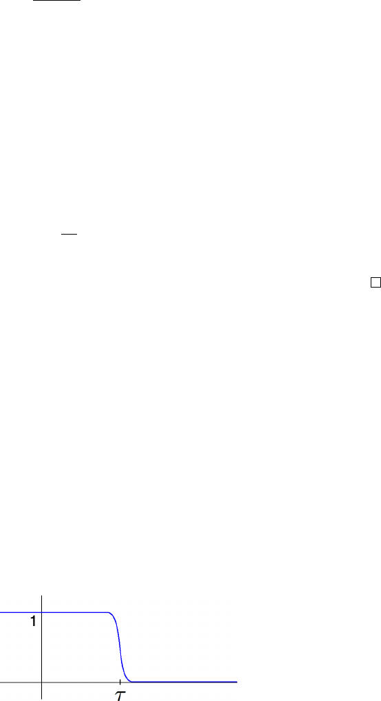
7.2 Slepian’s inequality 165
Consider a twice-differentiable function f
:
R
n
→ R such that
∂
2
f
∂x
i
∂x
j
≥ 0 for all i ̸= j.
Then
E f(X) ≥ E f(Y ),
assuming both expectations exist and are finite.
Proof The assumptions imply that the entries of the covariance matrices Σ
X
and Σ
Y
of X and Y satisfy
Σ
X
ii
= Σ
Y
ii
and Σ
X
ij
≥ Σ
Y
ij
.
for all i, j = 1, . . . , n. We can assume that X and Y are independent. (Why?)
Apply Lemma 7.2.7 and using our assumptions, we conclude that
d
du
E f(Z(u)) ≥ 0,
so E f (Z(u)) increases in u. Then E f (Z(1)) = E f(X) is at least as large as
E f(Z(0)) = E f(Y ). This completes the proof.
Now we are ready to prove Slepian’s inequality, Theorem 7.2.1. Let us state
and prove it in the equivalent form for Gaussian random vectors.
Theorem 7.2.9 (Slepian’s inequality). Let X and Y be Gaussian random vectors
as in Lemma 7.2.8. Then for every τ ≥ 0 we have
P
max
i≤n
X
i
≥ τ
≤ P
max
i≤n
Y
i
≥ τ
.
Consequently,
E max
i≤n
X
i
≤ E max
i≤n
Y
i
.
Proof Let h
:
R → [0, 1] be a twice-differentiable, non-increasing approximation
to the indicator function of the interval (−∞, τ):
h(x) ≈ 1
(−∞,τ)
,
see Figure 7.2. Define the function f
:
R
n
→ R by
Figure 7.2 The function h(x) is a smooth, non-increasing approximation to
the indicator function 1
(−∞,τ)
.

166 Random processes
f(x) = h(x
1
) ···h(x
n
).
Then f(x) is an approximation to the indicator function
f(x) ≈ 1
{max
i
x
i
<τ}
.
We are looking to apply the functional form of Slepian’s inequality, Lemma 7.2.8,
for f(x). To check the assumptions of this result, note that for i ̸= j we have
∂
2
f
∂x
i
∂x
j
= h
′
(x
i
)h
′
(x
j
) ·
Y
k̸∈{i,j}
h(x
k
).
The first two factors are non-positive and the others are non-negative by the
assumption. Thus the second derivative is non-negative, as required.
It follows that
E f(X) ≥ E f(Y ).
By approximation, this implies
P
max
i≤n
X
i
< τ
≥ P
max
i≤n
Y
i
< τ
.
This proves the first part of the conclusion. The second part follows using the
integral identity in Lemma 1.2.1, see Exercise 7.2.10.
Exercise 7.2.10. K Using the integral identity in Exercise 1.2.2, deduce the
second part of Slepian’s inequality (comparison of expectations).
7.2.3 Sudakov-Fernique’s and Gordon’s inequalities
Slepian’s inequality has two assumptions on the processes (X
t
) and (Y
t
) in (7.2):
the equality of variances and the dominance of increments. We now remove the
assumption on the equality of variances, and still be able to obtain (7.4). This
more practically useful result is due to Sudakov and Fernique.
Theorem 7.2.11 (Sudakov-Fernique’s inequality). Let (X
t
)
t∈T
and (Y
t
)
t∈T
be
two mean zero Gaussian processes. Assume that for all t, s ∈ T , we have
E(X
t
− X
s
)
2
≤ E(Y
t
− Y
s
)
2
.
Then
E sup
t∈T
X
t
≤ E sup
t∈T
Y
t
.
Proof It is enough to prove this theorem for Gaussian random vectors X and Y
in R
n
, just like we did for Slepian’s inequality in Theorem 7.2.9. We again deduce
the result from Gaussian Interpolation Lemma 7.2.7. But this time, instead of
choosing f(x) that approximates the indicator function of {max
i
x
i
< τ}, we
want f(x) to approximate max
i
x
i
.

7.2 Slepian’s inequality 167
To this end, let β > 0 be a parameter and define the function
5
f(x)
:
=
1
β
log
n
X
i=1
e
βx
i
. (7.11)
A quick check shows that
f(x) → max
i≤n
x
i
as β → ∞.
(Do this!) Substituting f (x) into the Gaussian interpolation formula (7.8) and
simplifying the expression shows that
d
du
E f(Z(u)) ≤ 0 for all u (see Exer-
cise 7.2.12 below). The proof can then be completed just like the proof of Slepian’s
inequality.
Exercise 7.2.12. KKK Show that
d
du
E f(Z(u)) ≤ 0 in Sudakov-Fernique’s
Theorem 7.2.11.
Hint: Differentiate f and check that
∂f
∂x
i
=
e
βx
i
P
k
e
βx
k
=
:
p
i
(x) and
∂
2
f
∂x
i
∂x
j
= β
δ
ij
p
i
(x) − p
i
(x)p
j
(x)
where δ
ij
is the Kronecker delta, which equals 1 is i = j and 0 otherwise. Next, check the following
numeric identity:
If
n
X
i=1
p
i
= 1 then
n
X
i,j=1
σ
ij
(δ
ij
p
i
− p
i
p
j
) =
1
2
X
i̸=j
(σ
ii
+ σ
jj
− 2σ
ij
)p
i
p
j
.
Use Gaussian interpolation formula 7.2.7. Simplify the expression using the identity above with σ
ij
=
Σ
X
ij
− Σ
Y
ij
and p
i
= p
i
(Z(u)). Deduce that
d
du
E f (Z(u)) =
β
4
X
i̸=j
h
E(X
i
− X
j
)
2
− E(Y
i
− Y
j
)
2
i
E p
i
(Z(u)) p
j
(Z(u)).
By the assumptions, this expression is non-positive.
Exercise 7.2.13 (Gaussian contraction inequality). KK The following is a
Gaussian version of Talagrand’s contraction principle we proved in Exercise 6.7.7.
Consider a bounded subset T ⊂ R
n
, and let g
1
, . . . , g
n
be independent N(0, 1)
random variables. Let ϕ
i
:
R → R be contractions, i.e. Lipschitz functions with
∥ϕ
i
∥
Lip
≤ 1. Prove that
E sup
t∈T
n
X
i=1
g
i
ϕ
i
(t
i
) ≤ E sup
t∈T
n
X
i=1
g
i
t
i
.
Hint: Use Sudakov-Fernique’s inequality.
Exercise 7.2.14 (Gordon’s inequality). KKK Prove the following extension of
Slepian’s inequality due to Y. Gordon. Let (X
ut
)
u∈U, t∈T
and Y = (Y
ut
)
u∈U, t∈T
be
5
The motivation for considering this form of f (x) comes from statistical mechanics, where the right
side of (7.11) can be interpreted as a log-partition function and β as the inverse temperature.

168 Random processes
two mean zero Gaussian processes indexed by pairs of points (u, t) in a product
set U × T . Assume that we have
E X
2
ut
= E Y
2
ut
, E(X
ut
− X
us
)
2
≤ E(Y
ut
− Y
us
)
2
for all u, t, s;
E(X
ut
− X
vs
)
2
≥ E(Y
ut
− Y
vs
)
2
for all u ̸= v and all t, s.
Then for every τ ≥ 0 we have
P
(
inf
u∈U
sup
t∈T
X
ut
≥ τ
)
≤ P
(
inf
u∈U
sup
t∈T
Y
ut
≥ τ
)
.
Consequently,
E inf
u∈U
sup
t∈T
X
ut
≤ E inf
u∈U
sup
t∈T
Y
ut
. (7.12)
Hint: Use Gaussian Interpolation Lemma 7.2.7 for f(x) =
Q
i
1 −
Q
j
h(x
ij
)
where h(x) is an approx-
imation to the indicator function 1
{x≤τ}
, as in the proof of Slepian’s inequality.
Similarly to Sudakov-Fernique’s inequality, it is possible to remove the assump-
tion of equal variances from Gordon’s theorem, and still be able to derive (7.12).
We do not prove this result.
7.3 Sharp bounds on Gaussian matrices
We illustrate Gaussian comparison inequalities that we just proved with an ap-
plication to random matrices. In Section 4.6, we studied m ×n random matrices
A with independent, sub-gaussian rows. We used the ε-net argument to control
the norm of A as follows:
E ∥A∥ ≤
√
m + C
√
n
where C is a constant. (See Exercise 4.6.3.) We now use Sudakov-Fernique’s
inequality to improve upon this bound for Gaussian random matrices, showing
that it holds with sharp constant C = 1.
Theorem 7.3.1 (Norms of Gaussian random matrices). Let A be an m×n matrix
with independent N(0, 1) entries. Then
E ∥A∥ ≤
√
m +
√
n.
Proof We can realize the norm of A as a supremum of a Gaussian process.
Indeed,
∥A∥ = max
u∈S
n−1
, v∈S
m−1
⟨Au, v⟩ = max
(u,v)∈T
X
uv
where T denotes the product set S
n−1
× S
m−1
and
X
uv
:
= ⟨Au, v⟩ ∼ N(0, 1).
(Check!)

7.3 Sharp bounds on Gaussian matrices 169
To apply Sudakov-Fernique’s comparison inequality (Theorem 7.2.11), let us
compute the increments of the process (X
uv
). For any (u, v), (w, z) ∈ T , we have
E(X
uv
− X
wz
)
2
= E
⟨Au, v⟩− ⟨Aw, z⟩
2
= E
X
i,j
A
ij
(u
j
v
i
− w
j
z
i
)
2
=
X
i,j
(u
j
v
i
− w
j
z
i
)
2
(by independence, mean 0, variance 1)
= ∥uv
T
− wz
T
∥
2
F
≤ ∥u − w∥
2
2
+ ∥v − z∥
2
2
(see Exercise 7.3.2 below).
Let us define a simpler Gaussian process (Y
uv
) with similar increments as fol-
lows:
Y
uv
:
= ⟨g, u⟩ + ⟨h, v⟩, (u, v) ∈ T,
where
g ∼ N(0, I
n
), h ∼ N(0, I
m
)
are independent Gaussian vectors. The increments of this process are
E(Y
uv
− Y
wz
)
2
= E
⟨g, u − w⟩ + ⟨h, v − z⟩
2
= E ⟨g, u − w⟩
2
+ E ⟨h, v − z⟩
2
(by independence, mean 0)
= ∥u − w∥
2
2
+ ∥v − z∥
2
2
(since g, h are standard normal).
Comparing the increments of the two processes, we see that
E(X
uv
− X
wz
)
2
≤ E(Y
uv
− Y
wz
)
2
for all (u, v), (w, z) ∈ T,
as required in Sudakov-Fernique’s inequality. Applying Theorem 7.2.11, we obtain
E ∥A∥ = E sup
(u,v)∈T
X
uv
≤ E sup
(u,v)∈T
Y
uv
= E sup
u∈S
n−1
⟨g, u⟩ + E sup
v∈S
m−1
⟨h, v⟩
= E ∥g∥
2
+ E ∥h∥
2
≤ (E ∥g∥
2
2
)
1/2
+ (E ∥h∥
2
2
)
1/2
(by inequality (1.3) for L
p
norms)
=
√
n +
√
m (recall Lemma 3.2.4).
This completes the proof.
Exercise 7.3.2. KKK Prove the following bound used in the proof of Theo-
rem 7.3.1. For any vectors u, w ∈ S
n−1
and v, z ∈ S
m−1
, we have
∥uv
T
− wz
T
∥
2
F
≤ ∥u − w∥
2
2
+ ∥v − z∥
2
2
.
While Theorem 7.3.1 does not give any tail bound for ∥A∥, we can automat-
ically deduce a tail bound using concentration inequalities we studied in Sec-
tion 5.2.

170 Random processes
Corollary 7.3.3 (Norms of Gaussian random matrices: tails). Let A be an m×n
matrix with independent N(0, 1) entries. Then for every t ≥ 0, we have
P
n
∥A∥ ≥
√
m +
√
n + t
o
≤ 2 exp(−ct
2
).
Proof This result follows by combining Theorem 7.3.1 with the concentration
inequality in the Gauss space, Theorem 5.2.2.
To use concentration, let us view A as a long random vector in R
m×n
by
concatenating the rows. This makes A a standard normal random vector, i.e.
A ∼ N(0, I
nm
). Consider the function f(A)
:
= ∥A∥ that assigns to the vector A
the operator norm of the matrix A. We have
f(A) ≤ ∥A∥
2
,
where ∥A∥
2
is the Euclidean norm in R
m×n
. (This is the same as the Frobenius
norm of A, which dominates the operator norm of A.) This shows that A 7→ ∥A∥
is a Lipschitz function on R
m×n
, and its Lipschitz norm is bounded by 1. (Why?)
Then Theorem 5.2.2 yields
P
∥A∥ ≥ E ∥A∥ + t
≤ 2 exp(−ct
2
).
The bound on E ∥A∥ from Theorem 7.3.1 completes the proof.
Exercise 7.3.4 (Smallest singular values). KKK Use Gordon’s inequality stated
in Exercise 7.2.14 to obtain a sharp bound on the smallest singular value of an
m × n random matrix A with independent N(0, 1) entries:
E s
n
(A) ≥
√
m −
√
n.
Combine this result with concentration to show the tail bound
P
n
∥A∥ ≤
√
m −
√
n − t
o
≤ 2 exp(−ct
2
).
Hint: Relate the smallest singular value to the min-max of a Gaussian process:
s
n
(A) = min
u∈S
n−1
max
v∈S
m−1
⟨Au, v⟩.
Apply Gordon’s inequality (without the requirement of equal variances, which is noted below Exer-
cise 7.2.14) to show that
E s
n
(A) ≥ E ∥h∥
2
− E ∥g∥
2
where g ∼ N(0, I
n
), h ∼ N(0, I
m
).
Combine this with the fact that f (n)
:
= E ∥g∥
2
−
√
n is increasing in dimension n. (Take this fact for
granted; it can be proved by a tedious calculation.)
Exercise 7.3.5 (Symmetric random matrices). KKK Modify the arguments
above to bound the norm of a symmetric n ×n Gaussian random matrix A whose
entries above the diagonal are independent N(0, 1) random variables, and the
diagonal entries are independent N(0, 2) random variables. This distribution of
random matrices is called the Gaussian orthogonal ensemble (GOE). Show that
E ∥A∥ ≤ 2
√
n.
7.4 Sudakov’s minoration inequality 171
Next, deduce the tail bound
P
n
∥A∥ ≥ 2
√
n + t
o
≤ 2 exp(−ct
2
).
7.4 Sudakov’s minoration inequality
Let us return to studying general mean zero Gaussian processes (X
t
)
t∈T
. As we
observed in Remark 7.1.7, the increments
d(t, s)
:
= ∥X
t
− X
s
∥
L
2
=
E(X
t
− X
s
)
2
1/2
(7.13)
define a metric on the (otherwise abstract) index set T , which we called the
canonical metric.
The canonical metric d(t, s) determines the covariance function Σ(t, s), which
in turn determines the distribution of the process (X
t
)
t∈T
(recall Exercise 7.1.8
and Remark 7.1.11.) So in principle, we should be able to answer any question
about the distribution of a Gaussian process (X
t
)
t∈T
by looking at the geometry
of the metric space (T, d). Put plainly, we should be able to study probability via
geometry.
Let us then ask an important specific question. How can we evaluate the overall
magnitude of the process, namely
E sup
t∈T
X
t
, (7.14)
in terms of the geometry of (T, d)? This turns out to be a difficult problem, which
we start to study here and continue in Chapter 8.
In this section, we prove a useful lower bound on (7.14) in terms of the metric
entropy of the metric space (T, d). Recall from Section 4.2 that for ε > 0, the
covering number
N(T, d, ε)
is defined to be the smallest cardinality of an ε-net of T in the metric d. Equiva-
lently, N(T, d, ε) is the smallest number
6
of closed balls of radius ε whose union
covers T . Recall also that the logarithm of the covering number,
log
2
N(T, d, ε)
is called the metric entropy of T .
Theorem 7.4.1 (Sudakov’s minoration inequality). Let (X
t
)
t∈T
be a mean zero
Gaussian process. Then, for any ε ≥ 0, we have
E sup
t∈T
X
t
≥ cε
q
log N(T, d, ε).
where d is the canonical metric defined in (7.13).
6
If T does not admit a finite ε-net, we set N(T, d, ε) = ∞.

172 Random processes
Proof Let us deduce this result from Sudakov-Fernique’s comparison inequality
(Theorem 7.2.11). Assume that
N(T, d, ε) =
:
N
is finite; the infinite case will be considered in Exercise 7.4.2. Let N be a maximal
ε-separated subset of T . Then N is an ε-net of T (recall Lemma 4.2.6), and thus
|N| ≥ N.
Restricting the process to N, we see that it suffices to show that
E sup
t∈N
X
t
≥ cε
p
log N.
We can do it by comparing (X
t
)
t∈N
to a simpler Gaussian process (Y
t
)
t∈N
,
which we define as follows:
Y
t
:
=
ε
√
2
g
t
, where g
t
are independent N(0, 1) random variables.
To use Sudakov-Fernique’s comparison inequality (Theorem 7.2.11), we need to
compare the increments of the two processes. Fix two different points t, s ∈ N.
By definition, we have
E(X
t
− X
s
)
2
= d(t, s)
2
≥ ε
2
while
E(Y
t
− Y
s
)
2
=
ε
2
2
E(g
t
− g
s
)
2
= ε
2
.
(In the last line, we use that g
t
− g
s
∼ N(0, 2).) This implies that
E(X
t
− X
s
)
2
≥ E(Y
t
− Y
s
)
2
for all t, s ∈ N.
Applying Theorem 7.2.11, we obtain
E sup
t∈N
X
t
≥ E sup
t∈N
Y
t
=
ε
√
2
E max
t∈N
g
t
≥ cε
p
log N.
In the last inequality we used that the expected maximum of N standard normal
random variables is at least c
√
log N, see Exercise 2.5.11. The proof is complete.
Exercise 7.4.2 (Sudakov’s minoration for non-compact sets). KK Show that
if (T, d) is not relatively compact, that is if N(T, d, ε) = ∞ for some ε > 0, then
E sup
t∈T
X
t
= ∞.

7.4 Sudakov’s minoration inequality 173
7.4.1 Application for covering numbers in R
n
Sudakov’s minoration inequality can be used to estimate the covering numbers
of sets T ⊂ R
n
. To see how to do this, consider a canonical Gaussian process on
T , namely
X
t
:
= ⟨g, t⟩, t ∈ T, where g ∼ N(0, I
n
).
As we observed in Section 7.1.2, the canonical distance for this process is the
Euclidean distance in R
n
, i.e.
d(t, s) = ∥X
t
− X
s
∥
L
2
= ∥t − s∥
2
.
Thus Sudakov’s inequality can be stated as follows.
Corollary 7.4.3 (Sudakov’s minoration inequality in R
n
). Let T ⊂ R
n
. Then,
for any ε > 0, we have
E sup
t∈T
⟨g, t⟩ ≥ cε
q
log N(T, ε).
Here N(T, ε) is the covering number of T by Euclidean balls – the smallest
number of Euclidean balls with radii ε and centers in T that cover T , just like in
Section 4.2.1.
To give an illustration of Sudakov’s minoration, note that it yields (up to an
absolute constant) the same bound on the covering numbers of polytopes in R
n
that we gave in Corollary 0.0.4:
Corollary 7.4.4 (Covering numbers of polytopes). Let P be a polytope in R
n
with N vertices and whose diameter is bounded by 1. Then, for every ε > 0 we
have
N(P, ε) ≤ N
C/ε
2
.
Proof As before, by translation, we may assume that the radius of P is bounded
by 1. Denote by x
1
, . . . , x
N
the vertices of P . Then
E sup
t∈P
⟨g, t⟩ = E sup
i≤N
⟨g, x
i
⟩ ≤ C
p
log N.
The equality here follows since the maximum of the linear function on the convex
set P is attained at an extreme point, i.e. at a vertex of P . The bound is due
to Exercise 2.5.10, since ⟨g, x⟩ ∼ N(0, ∥x∥
2
2
) and ∥x∥
2
≤ 1. Substituting this into
Sudakov’s minoration inequality of Corollary 7.4.3 and simplifying, we complete
the proof.
Exercise 7.4.5 (Volume of polytopes). KKK Let P be a polytope in R
n
, which
has N vertices and is contained in the unit Euclidean ball B
n
2
. Show that
Vol(P )
Vol(B
n
2
)
≤
C log N
n
Cn
.
Hint: Use Proposition 4.2.12, Corollary 7.4.4 and optimize in ε.

174 Random processes
7.5 Gaussian width
In the previous section, we encountered an important quantity associated with a
general set T ⊂ R
n
. It is the magnitude of the canonical Gaussian process on T ,
i.e.
E sup
t∈T
⟨g, t⟩
where the expectation is taken with respect to the Gaussian random vector g ∼
N(0, I
n
). This quantity plays a central role in high-dimensional probability and
its applications. Let us give it a name and study its basic properties.
Definition 7.5.1. The Gaussian width of a subset T ⊂ R
n
is defined as
w(T)
:
= E sup
x∈T
⟨g, x⟩ where g ∼ N(0, I
n
).
One can think about Gaussian width w(T ) as one of the basic geometric quan-
tities associated with subsets of T ⊂ R
n
, such as volume and surface area. Several
variants of the definition of Gaussian width can be found in the literature, such
as
E sup
x∈T
|⟨g, x⟩|,
E sup
x∈T
⟨g, x⟩
2
1/2
, E sup
x,y∈T
⟨g, x − y⟩, etc.
These versions are equivalent, or almost equivalent, to w(T ) as we will see in
Section 7.6.
7.5.1 Basic properties
Proposition 7.5.2 (Gaussian width).
(a) w(T ) is finite if and only if T is bounded.
(b) Gaussian width is invariant under affine unitary transformations. Thus,
for every orthogonal matrix U and any vector y, we have
w(UT + y) = w(T ).
(c) Gaussian width is invariant under taking convex hulls. Thus,
w(conv(T )) = w(T ).
(d) Gaussian width respects Minkowski addition of sets and scaling. Thus, for
T, S ⊂ R
n
and a ∈ R we have
w(T + S) = w(T) + w(S); w(aT ) = |a|w(T ).
(e) We have
w(T) =
1
2
w(T − T ) =
1
2
E sup
x,y∈T
⟨g, x − y⟩.

7.5 Gaussian width 175
(f) (Gaussian width and diameter). We have
7
1
√
2π
· diam(T ) ≤ w(T) ≤
√
n
2
· diam(T ).
Proof Properties a–d are simple and will be checked in Exercise 7.5.3 below.
To prove property e, we use property d twice and get
w(T) =
1
2
w(T) + w(T )
=
1
2
w(T) + w(−T )
=
1
2
w(T − T ),
as claimed.
To prove the lower bound in property f, fix a pair of points x, y ∈ T . Then
both x − y and y − x lie in T − T , so by property e we have
w(T) ≥
1
2
E max
⟨x − y, g⟩, ⟨y −x, g⟩
=
1
2
E |⟨x − y, g⟩| =
1
2
r
2
π
∥x − y∥
2
.
The last identity follows since ⟨x − y, g⟩ ∼ N(0, ∥x−y∥
2
2
) and since E |X| =
p
2/π
for X ∼ N(0, 1). (Check!) It remains to take supremum over all x, y ∈ T , and the
lower bound in property f follows.
To prove the upper bound in property f, we again use property e to get
w(T) =
1
2
E sup
x,y∈T
⟨g, x − y⟩
≤
1
2
E sup
x,y∈T
∥g∥
2
∥x − y∥
2
≤
1
2
E ∥g∥
2
· diam(T ).
It remains to recall that E ∥g∥
2
≤ (E ∥g∥
2
2
)
1/2
=
√
n.
Exercise 7.5.3. KK Prove Properties a–d in Proposition 7.5.2.
Hint: Use rotation invariance of Gaussian distribution.
Exercise 7.5.4 (Gaussian width under linear transformations). KKK Show
that for any m × n matrix A, we have
w(AT) ≤ ∥A∥w(T ).
Hint: Use Sudakov-Fernique’s comparison inequality.
7.5.2 Geometric meaning of width
The notion of the Gaussian width of a set T ⊂ R
n
has a nice geometric meaning.
The width of T in the direction of a vector θ ∈ S
n−1
is the smallest width of the
slab that is formed by parallel hyperplanes orthogonal to θ and that contains T ;
see Figure 7.3. Analytically, the width in the direction of θ can be expressed as
7
Recall that the diameter of a set T ⊂ R
n
is defined as diam(T )
:
= sup{∥x − y∥
2
:
x, y ∈ T }.

176 Random processes
Figure 7.3 The width of a set T ⊂ R
n
in the direction of a unit vector θ.
sup
x,y∈T
⟨θ, x − y⟩.
(Check!) If we average the width over all unit directions θ, we obtain the quantity
E sup
x,y∈T
⟨θ, x − y⟩. (7.15)
Definition 7.5.5 (Spherical width). The spherical width
8
of a subset T ⊂ R
n
is
defined as
w
s
(T )
:
= E sup
x∈T
⟨θ, x⟩ where θ ∼ Unif(S
n−1
).
The quantity in (7.15) clearly equals w
s
(T − T ).
How different are the Gaussian and spherical widths of T ? The difference is in
the random vectors we use to do the averaging; they are g ∼ N(0, I
n
) for Gaussian
width and θ ∼ Unif(S
n−1
) for spherical width. Both g and θ are rotation invariant,
and, as we know, g is approximately
√
n longer than θ. This makes Gaussian
width just a scaling of the spherical width by approximately
√
n. Let us make
this relation more precise.
Lemma 7.5.6 (Gaussian vs. spherical widths). We have
(
√
n − C) w
s
(T ) ≤ w(T) ≤ (
√
n + C) w
s
(T ).
Proof Let us express the Gaussian vector g through its length and direction:
g = ∥g∥
2
·
g
∥g∥
2
=
:
rθ.
As we observed in Section 3.3.3, r and θ are independent and θ ∼ Unif(S
n−1
).
Thus
w(T) = E sup
x∈T
⟨rθ, x⟩ = (E r) · E sup
x∈T
⟨θ, x⟩ = E ∥g∥
2
· w
s
(T ).
It remains to recall that concentration of the norm implies that
E ∥g∥
2
−
√
n
≤ C,
see Exercise 3.1.4.
8
The spherical width is also called the mean width in the literature.

7.5 Gaussian width 177
7.5.3 Examples
Example 7.5.7 (Euclidean ball and sphere). The Gaussian width of the Eu-
clidean unit sphere and ball is
w(S
n−1
) = w(B
n
2
) = E ∥g∥
2
=
√
n ± C, (7.16)
where we used the result of Exercise 3.1.4. The spherical widths of these sets of
course equal 1.
Example 7.5.8 (Cube). The unit ball of the ℓ
∞
norm in R
n
is B
n
∞
= [−1, 1]
n
.
We have
w(B
n
∞
) = E ∥g∥
1
(check!)
= E |g
1
| · n =
r
2
π
· n. (7.17)
Comparing with (7.16), we see that Gaussian widths of the cube B
n
∞
and its
circumscribed ball
√
nB
n
2
have the same order n; see Figure 7.4a.
(a) The Gaussian widths of the cube and
its circumscribed ball are of the same or-
der n.
(b) The Gaussian widths of B
n
1
and its in-
scribed ball are almost of the same order.
Figure 7.4 Gaussian widths of some classical sets in R
n
.
Example 7.5.9 (ℓ
1
ball). The unit ball of the ℓ
1
norm in R
n
is the set
B
n
1
= {x ∈ R
n
:
∥x∥
1
≤ 1}
which is sometimes called a cross-polytope; see Figure 7.5 for an illustration. The
Gaussian width of the ℓ
1
ball can be bounded as follows:
c
p
log n ≤ w(B
n
1
) ≤ C
p
log n. (7.18)
To see this, check that
w(B
n
1
) = E ∥g∥
∞
= E max
i≤n
|g
i
|.
Then the bounds (7.18) follow from Exercises 2.5.10 and 2.5.11. Note that the
Gaussian widths of the ℓ
1
ball B
n
1
and its inscribed ball
1
√
n
B
n
2
have almost same
order (up to a logarithmic factor); see Figure 7.4b.

178 Random processes
Figure 7.5 The unit ball of the ℓ
1
norm in R
n
, denoted B
n
1
, is a diamond in
dimension n = 2 (left) and a regular octahedron in dimension n = 3 (right).
Exercise 7.5.10 (Finite point sets). K Let T be a finite set of points in R
n
.
Check that
w(T) ≤ C
q
log |T | · diam(T ).
Hint: Argue like in the proof of Corollary 7.4.4.
Exercise 7.5.11 (ℓ
p
balls). KKK Let 1 ≤ p < ∞. Consider the unit ball of
the ℓ
p
norm in R
n
:
B
n
p
:
=
x ∈ R
n
:
∥x∥
p
≤ 1
.
Check that
w(B
n
p
) ≤ C
p
p
′
n
1/p
′
.
Here p
′
denotes the conjugate exponent for p, which is defined by the equation
1
p
+
1
p
′
= 1.
7.5.4 Surprising behavior of width in high dimensions
According to our computation in Example 7.5.9, the spherical width of B
n
1
is
w
s
(B
n
1
) ≍
r
log n
n
.
Surprisingly, it is much smaller than the diameter of B
n
1
, which equals 2! Further,
as we already noted, the Gaussian width of B
n
1
is roughly the same (up to a
logarithmic factor) as the Gaussian width of its inscribed Euclidean ball
1
√
n
B
n
2
.
This again might look strange. Indeed, the cross-polytope B
n
1
looks much larger
than its inscribed ball whose diameter is
2
√
n
! Why does Gaussian width behave
this way?
Let us try to give an intuitive explanation. In high dimensions, the cube B
n
∞
has so many vertices (2
n
) that in most directions it extends to a radius close to
√
n, so it nearly covers the volume of the enclosing ball. In fact, the volumes of
the cube and its circumscribed ball are both of the order C
n
, so these sets are
not far from each other from the volumetric point of view. So it should not be

7.6 Stable dimension, stable rank, and Gaussian complexity 179
very surprising to see that the Gaussian widths of the cube and its circumscribed
ball are also of the same order.
The octahedron B
n
1
has much fewer vertices (2n) than the cube. A random
direction θ in R
n
is likely to be almost orthogonal to all of them. So the width of
B
n
1
in the direction of θ is not significantly influenced by the presence of vertices.
What really determines the width of B
n
1
is its “bulk”, which is the inscribed
Euclidean ball.
A similar picture can be seen from the volumetric viewpoint. There are so few
vertices in B
n
1
that the regions near them contain very little volume. The bulk
of the volume of B
n
1
lies much closer to the origin, not far from the inscribed
Euclidean ball. Indeed, one can check that the volumes of B
n
1
and its inscribed
ball are both of the order of (C/n)
n
. So from the volumetric point of view, the
octahedron B
n
1
is similar to its inscribed ball; Gaussian width gives the same
result.
We can illustrate this phenomenon on Figure 7.6b that shows a “hyperbolic”
picture of B
n
1
that is due to V. Milman. Such pictures capture the bulk and
outliers very well, but unfortunately they may not accurately show convexity.
(a) General convex set (b) The octahedron B
n
1
Figure 7.6 An intuitive, hyperbolic picture of a convex body in R
n
. The
bulk is a round ball that contains most of the volume.
7.6 Stable dimension, stable rank, and Gaussian complexity
The notion of Gaussian width will help us to introduce a more robust version of
the classical notion of dimension. The usual, linear algebraic, dimension dim T
of a subset T ⊂ R
n
is the smallest dimension of an affine subspace E ⊂ R
n
that contains T . The linear algebraic dimension is unstable: it can significantly
change (usually upwards) under a small perturbation of T . A more stable version
of dimension can be defined based on the concept of Gaussian width.
In this section, it will be more convenient to work with a closely related squared
version of the Gaussian width:
h(T )
2
:
= E sup
t∈T
⟨g, t⟩
2
, where g ∼ N(0, I
n
). (7.19)

180 Random processes
It is not difficult to see that the squared and usual versions of the Gaussian width
are equivalent up to constant factor:
Exercise 7.6.1 (Equivalence). KKK Check that
w(T − T ) ≤ h(T − T ) ≤ w(T − T ) + C
1
diam(T ) ≤ Cw(T − T ).
In particular, we have
2w(T) ≤ h(T − T ) ≤ 2C w(T ). (7.20)
Hint: Use Gaussian concentration to prove the upper bound.
Definition 7.6.2 (Stable dimension). For a bounded set T ⊂ R
n
, the stable
dimension of T is defined as
d(T )
:
=
h(T − T )
2
diam(T )
2
≍
w(T)
2
diam(T )
2
.
The stable dimension is always bounded by the algebraic dimension:
Lemma 7.6.3. For any set T ⊂ R
n
, we have
d(T ) ≤ dim(T ).
Proof Let dim T = k; this means that T lies in some subspace E ⊂ R
n
of
dimension k. By rotation invariance, we can assume that E is the coordinate
subspace, i.e. E = R
k
. (Why?) By definition, we have
h(T − T )
2
= E sup
x,y∈T
⟨g, x − y⟩
2
.
Since x −y ∈ R
k
and ∥x −y∥
2
≤ diam(T ), we have x −y = diam(T ) · z for some
z ∈ B
k
2
. Thus the quantity above is bounded by
diam(T )
2
· E sup
z∈B
k
2
⟨g, z⟩
2
= diam(T )
2
· E ∥g
′
∥
2
2
= diam(T )
2
· k
where g
′
∼ N(0, I
k
) is a standard Gaussian random vector in R
k
. The proof is
complete.
The inequality d(T ) ≤ dim(T ) is in general sharp:
Exercise 7.6.4. K Show that if T is a Euclidean ball in any subspace of R
n
,
then
d(T ) = dim(T ).
However, in many cases the stable dimension can be much smaller than the
algebraic dimension:
Example 7.6.5. Let T be a finite set of points in R
n
. Then
d(T ) ≤ C log |T |.
This follows from the bound on the Gaussian width of T in Exercise 7.5.10.

7.6 Stable dimension, stable rank, and Gaussian complexity 181
7.6.1 Stable rank
The stable dimension is more robust than the algebraic dimension. Indeed, small
perturbation of a set T leads to small perturbation of Gaussian width and the
diameter of T , and thus the stable dimension d(T ).
To give an example, consider the unit Euclidean ball B
n
2
, for which both al-
gebraic and stable dimensions equal n. Let us decrease one of the axes of B
n
2
gradually from 1 to 0. The algebraic dimension will stay at n through this pro-
cess and then instantly jump to n − 1. The stable dimension instead decreases
gradually from n to n −1. To see how exactly stable dimension decreases, do the
following computation.
Exercise 7.6.6 (Ellipsoids). KK Let A be an m ×n matrix, and let B
n
2
denote
the unit Euclidean ball. Check that the squared mean width of the ellipsoid AB
n
2
is the Frobenius norm of A, i.e.
h(AB
n
2
) = ∥A∥
F
.
Deduce that the stable dimension of the ellipsoid AB
n
2
equals
d(AB
n
2
) =
∥A∥
2
F
∥A∥
2
. (7.21)
This example relates the stable dimension to the notion of stable rank of ma-
trices, which is a robust version of the classical, linear algebraic rank.
Definition 7.6.7 (Stable rank). The stable rank of an m ×n matrix A is defined
as
r(A)
:
=
∥A∥
2
F
∥A∥
2
.
The robustness of stable rank makes it a useful quantity in numerical linear
algebra. The usual, algebraic, rank is the algebraic dimension of the image of A;
in particular
rank(A) = dim(AB
n
2
).
Similarly, (7.21) shows that the stable rank is the statistical dimension of the
image:
r(A) = d(AB
n
2
).
Finally, note that the stable rank is always bounded by the usual rank:
r(A) ≤ rank(A).
(Check this!)
7.6.2 Gaussian complexity
Let us mention one more cousin of the Gaussian width where instead of squaring
⟨g, x⟩ as in (7.19) we take absolute value.

182 Random processes
Definition 7.6.8. The Gaussian complexity of a subset T ⊂ R
n
is defined as
γ(T )
:
= E sup
x∈T
|⟨g, x⟩| where g ∼ N(0, I
n
).
Obviously, we have
w(T) ≤ γ(T ),
and equality holds if T is origin-symmetric, i.e. if T = −T . Since T −T is origin-
symmetric, property e of Proposition 7.5.2 implies that
w(T) =
1
2
w(T − T ) =
1
2
γ(T − T ). (7.22)
In general, Gaussian width and complexity may be quite different. For example,
if T consists of a single nonzero point, then w(T ) = 0 but γ(T ) > 0. Still, these
two quantities are very closely related:
Exercise 7.6.9 (Gaussian width vs. Gaussian complexity). KKK Consider a
set T ⊂ R
n
and a point y ∈ T . Show that
1
3
w(T) + ∥y∥
2
≤ γ(T ) ≤ 2
w(T) + ∥y∥
2
This implies in particular that Gaussian width and Gaussian complexity are
equivalent for any set T that contains the origin:
w(T) ≤ γ(T ) ≤ 2w(T).
(It is fine if you prove the inequalities above with other absolute constants instead
of 2 and 1/3.)
7.7 Random projections of sets
This section will illustrate the importance of the notion of Gaussian (and spheri-
cal) width in dimension reduction problems. Consider a set T ⊂ R
n
and project it
onto a random m-dimensional subspace in R
n
(chosen uniformly from the Grass-
manian G
n,m
); see Figure 5.2 for illustration. In applications, we might think of
T as a data set and P as a means of dimension reduction. What can we say about
the size (diameter) of the projected set P T ?
For a finite set T , Johnson-Lindenstrauss Lemma (Theorem 5.3.1) states that
as long as
m ≳ log |T |, (7.23)
the random projection P acts essentially as a scaling of T . Namely, P shrinks all
distances between points in T by a factor ≈
p
m/n. In particular,
diam(P T ) ≈
r
m
n
diam(T ). (7.24)
If the cardinality of T is too large or infinite, then (7.24) may fail. For example,

7.7 Random projections of sets 183
if T = B
n
2
is a Euclidean ball then no projection can shrink the size of T at all,
and we have
diam(P T ) = diam(T ). (7.25)
What happens for a general set T ? The following result states that a random
projection shrinks T as in (7.24), but it can not shrink it beyond the spherical
width of T .
Theorem 7.7.1 (Sizes of random projections of sets). Consider a bounded set
T ⊂ R
n
. Let P be a projection in R
n
onto a random m-dimensional subspace
E ∼ Unif(G
n,m
). Then, with probability at least 1 − 2e
−m
, we have
diam(P T ) ≤ C
w
s
(T ) +
r
m
n
diam(T )
.
To prove of this result, we pass to an equivalent probabilistic model, just like
we did in the proof of Johnson-Lindenstrauss Lemma (see the proof of Propo-
sition 5.3.2). First, a random subspace E ⊂ R
n
can be realized by a random
rotation of some fixed subspace, such as R
m
. Next, instead of fixing T and ran-
domly rotating the subspace, we can fix the subspace and randomly rotate T .
The following exercise makes this reasoning more formal.
Exercise 7.7.2 (Equivalent models for random projections). KK Let P be a
projection in R
n
onto a random m-dimensional subspace E ∼ Unif(G
n,m
). Let Q
be an m × n matrix obtained by choosing the first m rows of a random n × n
matrix U ∼ Unif(O(n)) drawn uniformly from the orthogonal group.
(a) Show that for any fixed point x ∈ R
n
,
∥P x∥
2
and ∥Qx∥
2
have the same distribution.
Hint: Use the singular value decomposition of P .
(b) Show that for any fixed point z ∈ S
m−1
,
Q
T
z ∼ Unif(S
n−1
).
In other words, the map Q
T
acts as a random isometric embedding of R
m
into R
n
. Hint: It is enough to check the rotation invariance of the distribution of Q
T
z.
Proof of Theorem 7.7.1. Our argument is another example of an ε-net argu-
ment. Without loss of generality, we may assume that diam(T ) ≤ 1. (Why?)
Step 1: Approximation. By Exercise 7.7.2, it suffices to prove the theorem
for Q instead of P . So we are going to bound
diam(QT ) = sup
x∈T −T
∥Qx∥
2
= sup
x∈T −T
max
z∈S
m−1
⟨Qx, z⟩.
Similarly to our older arguments (for example, in the proof of Theorem 4.4.5 on
random matrices), we discretize the sphere S
m−1
. Choose an (1/2)-net N of S
m−1
so that
|N| ≤ 5
m
;

184 Random processes
this is possible to do by Corollary 4.2.13. We can replace the supremum over the
sphere S
m−1
by the supremum over the net N paying a factor 2:
diam(QT ) ≤ 2 sup
x∈T −T
max
z∈N
⟨Qx, z⟩ = 2 max
z∈N
sup
x∈T −T
D
Q
T
z, x
E
. (7.26)
(Recall Exercise 4.4.2.) We first control the quantity
sup
x∈T −T
D
Q
T
z, x
E
(7.27)
for a fixed z ∈ N and with high probability, and then take union bound over all
z.
Step 2: Concentration. So, let us fix z ∈ N. By Exercise 7.7.2, Q
T
z ∼
Unif(S
n−1
). The expectation of (7.27) can be realized as the spherical width:
E sup
x∈T −T
D
Q
T
z, x
E
= w
s
(T − T ) = 2w
s
(T ).
(The last identity is the spherical version of a similar property of the Gaussian
width, see part e of Proposition 7.5.2.)
Next, let us check that (7.27) concentrates nicely around its mean 2w
s
(T ). For
this, we can use the concentration inequality (5.6) for Lipschitz functions on the
sphere. Since we assumed that diam(T ) ≤ 1 in the beginning, one can quickly
check that the function
θ 7→ sup
x∈T −T
⟨θ, x⟩
is a Lipschitz function on the sphere S
n−1
, and its Lipschitz norm is at most 1.
(Do this!) Therefore, applying the concentration inequality (5.6), we obtain
P
(
sup
x∈T −T
D
Q
T
z, x
E
≥ 2w
s
(T ) + t
)
≤ 2 exp(−cnt
2
).
Step 3: Union bound. Now we unfix z ∈ N by taking the union bound over
N. We get
P
(
max
z∈N
sup
x∈T −T
D
Q
T
z, x
E
≥ 2w
s
(T ) + t
)
≤ |N| · 2 exp(−cnt
2
) (7.28)
Recall that |N| ≤ 5
m
. Then, if we choose
t = C
r
m
n
with C large enough, the probability in (7.28) can be bounded by 2e
−m
. Then
(7.28) and (7.26) yield
P
(
1
2
diam(QT ) ≥ 2w
s
(T ) + C
r
m
n
)
≤ e
−m
.
This proves Theorem 7.7.1.

7.7 Random projections of sets 185
Exercise 7.7.3 (Gaussian projection). KKK Prove a version of Theorem 7.7.1
for m × n Gaussian random matrix G with independent N(0, 1) entries. Specifi-
cally, show that for any bounded set T ⊂ R
n
, we have
diam(GT ) ≤ C
h
w(T) +
√
m diam(T )
i
with probability at least 1 − 2e
−m
. Here w(T ) is the Gaussian width of T .
Exercise 7.7.4 (The reverse bound). KKK Show that the bound in Theo-
rem 7.7.1 is optimal: prove the reverse bound
E diam(P T ) ≥ c
w
s
(T ) +
r
m
n
diam(T )
for all bounded sets T ⊂ R
n
.
Hint: To obtain the bound E diam(P T ) ≳ w
s
(T ), reduce P to a one-dimensional projection by dropping
terms from the singular value decomposition of P . To obtain the bound E diam(P T ) ≥
p
m
n
diam(T ),
argue about a pair of points in T .
Exercise 7.7.5 (Random projections of matrices). KK Let A be an n × k
matrix.
(a) Let P be a projection in R
n
onto a random m-dimensional subspace chosen
uniformly in G
n,m
. Show that with probability at least 1 − 2e
−m
, we have
∥P A∥ ≤ C
1
√
n
∥A∥
F
+
r
m
n
∥A∥
.
(b) Let G be an m × n Gaussian random matrix with independent N (0, 1)
entries. Show that with probability at least 1 − 2e
−m
, we have
∥GA∥ ≤ C
∥A∥
F
+
√
m ∥A∥
.
Hint: Express the operator norm of P A to the diameter of the ellipsoid P (AB
k
2
), and use Theorem 7.7.1
in part 1 and Exercise 7.7.3 in part 2.
7.7.1 The phase transition
Let us pause to take a closer look at the bound Theorem 7.7.1 gives. We can
equivalently write it as
diam(P T ) ≤ C max
w
s
(T ),
r
m
n
diam(T )
.
Let us compute the dimension m for which the phase transition occurs between
the two terms w
s
(T ) and
p
m
n
diam(T ). Setting them equal to each other and

186 Random processes
solving for m, we find that the phase transition happens when
m =
(
√
n w
s
(T ))
2
diam(T )
2
≍
w(T)
2
diam(T )
2
(pass to Gaussian width using Lemma 7.5.6)
≍ d(T ) (by Definition 7.6.2 of stable dimension).
So we can express the conclusion of Theorem 7.7.1 as follows:
diam(P T ) ≤
C
r
m
n
diam(T ), if m ≥ d(T )
Cw
s
(T ), if m ≤ d(T ).
Figure 7.7 shows a graph of diam(P T ) as a function of the dimension m.
Figure 7.7 The diameter of a random m-dimensional projection of a set T
as a function of m.
For large m, the random m-dimensional projection shrinks T by the factor
∼
p
m/n, just like we have seen in (7.24) in the context of Johnson-Lindenstrauss
lemma. However, when the dimension m drops below the stable dimension d(T ),
the shrinking stops – it levels off at the spherical width w
s
(T ). We saw an example
of this in (7.25), where a Euclidean ball can not be shrunk by a projection.
7.8 Notes
There are several introductory books on random processes (also called stochastic
processes) and in particular on Brownian motion, for example [37, 127, 182, 156].
Slepian’s inequality (Theorem 7.2.1) is originally due to D. Slepian [186, 187];
modern proofs can be found e.g. in [130, Corollary 3.12], [3, Section 2.2], [212, Sec-
tion 6.1], [105], [111]. Sudakov-Fernique inequality (Theorem 7.2.11) is attributed
to V. N. Sudakov [193, 194] and X. Fernique [75]. Our presentation of the proofs

7.8 Notes 187
of Slepian’s and Sudakov-Fernique’s inequalities in Section 7.2 is based on the ap-
proach of J.-P. Kahane [111] and a smoothing argument of S. Chatterjee (see [3,
Section 2.2]), and it follows [212, Section 6.1]. A more general version of Gaussian
contraction inequality in Exercise 7.2.13 can be found in [130, Corollary 3.17].
Gordon’s inequality we stated in Exercise 7.2.14 and its extensions can be found
in [84, 85, 88, 111]. Applications of Gordon’s inequality for convex optimization
can be found e.g. in [202, 200, 203].
The relevance of comparison inequalities to random matrix theory was noticed
by S. Szarek. The applications we presented in Section 7.3 can derived from the
work of Y. Gordon [84]. Our presentation there follows the argument in [59,
Section II.c], which is also reproduced in [222, Section 5.3.1].
Sudakov’s minoration inequality (Theorem 7.4.1) was originally proved by
V. N. Sudakov. Our presentation follows [130, Theorem 3.18]; see [11, Section 4.2]
for an alternative proof via duality. The volume bound in Exercise 7.4.5 is almost
best possible, but not quite. A slightly stronger bound
Vol(P )
Vol(B
n
2
)
≤
C log(1 + N/n)
n
n/2
can be deduced in exactly the same way, if we use from the stronger bound on
the covering numbers given in Exercise 0.0.6. This result is known and is best
possible up to a constant C [50, Section 3].
Gaussian width and its cousins, which we introduce in Section 7.5, was origi-
nally introduced in geometric functional analysis and asymptotic convex geome-
try [11, 150]. More recently, starting from [178], the role of Gaussian width was
recognized in applications to signal processing and high-dimensional statistics
[189, 161, 190, 52, 169, 9, 201, 163]; see also [223, Section 3.5], [132]. In Sec-
tion 7.5.4 we noted some surprising geometric phenomena in high dimensions; to
learn more about them see the preface of [11] and [13].
The notion of stable dimension d(T ) of a set T ⊂ R
n
introduced in Section 7.6
seems to be new. In the special case where T is a closed convex cone, the squared
version of Gaussian width h(T ) defined in (7.19) is often called statistical dimen-
sion of T in the literature on signal recovery [140, 9, 163].
The notion of stable rank r(A) = ∥A∥
2
F
/∥A∥
2
of a matrix A (also called ef-
fective, or numerical rank) seems to appear for the first time in [177]. In some
literature (e.g. [222, 119]) the quantity
k(Σ) =
tr(Σ)
∥Σ∥
is also called the stable rank of a symmetric positive semidefinite matrix Σ; we
call k(Σ) the intrinsic dimension following [207, Definition 7.1.1]. Note that we
used the quantity k(Σ) in covariance estimation (see Remark 5.6.3). Clearly, if
Σ = A
T
A or Σ = AA
T
then
k(Σ) = r(A).

8
Chaining
This chapter presents some of the central concepts and methods to bound random
processes. Chaining is a powerful and general technique to prove uniform bounds
on a random process (X
t
)
t∈T
. We present a basic version of chaining method in
Section 8.1. There we prove Dudley’s bound on random processes in terms of
covering numbers of T . In Section 8.2, we give applications of Dudley’s inequality
to Monte-Carlo integration and a uniform law of large numbers.
In Section 8.3 we show how to find bounds for random processes in terms of the
VC dimension of T . Unlike covering numbers, VC dimension is a combinatorial
rather than geometric quantity. It plays important role in problems of statistical
learning theory, which we discuss in Section 8.4.
As we will see in Section 8.1.2), the bounds on empirical processes in terms of
covering numbers – Sudakov’s inequality from Section 7.4 and Dudley’s inequality
– are sharp up to a logarithmic factor. The logarithmic gap is insignificant in many
applications, but it can not be removed in general. A sharper bound on random
processes, without any logarithmic gap, can be given in terms of the so-called
M. Talagrand’s functional γ
2
(T ), which captures the geometry of T better than
the covering numbers. We prove a sharp upper bound is Section 8.5 by a refined
chaining argument, often called “generic chaining”.
A matching lower bound due to M. Talagrand is more difficult to obtain; we
will state it without proof in Section 8.6. The resulting sharp, two-sided bound on
random processes is known as the majorizing measure theorem (Theorem 8.6.1).
A very useful consequence of this result is Talagrand’s comparison inequality
(Corollary 8.6.2), which generalizes Sudakov-Fernique’s inequality for all sub-
gaussian random processes.
Talagrand’s comparison inequality has many applications. One of them, Chevet’s
inequality, will be discussed in Section 8.7; others will appear later.
8.1 Dudley’s inequality
Sudakov’s minoration inequality that we studied in Section 7.4 gives a lower
bound on the magnitude
E sup
t∈T
X
t
189

190 Chaining
of a Gaussian random process (X
t
)
t∈T
in terms of the metric entropy of T . In
this section, we obtain a similar upper bound.
This time, we are able to work not just with Gaussian processes but with more
general processes with sub-gaussian increments.
Definition 8.1.1 (Sub-gaussian increments). Consider a random process (X
t
)
t∈T
on a metric space (T, d). We say that the process has sub-gaussian increments if
there exists K ≥ 0 such that
∥X
t
− X
s
∥
ψ
2
≤ Kd(t, s) for all t, s ∈ T. (8.1)
Example 8.1.2. Let (X
t
)
t∈T
be a Gaussian process on an abstract set T . Define
a metric on T by
d(t, s)
:
= ∥X
t
− X
s
∥
L
2
, t, s ∈ T.
Then (X
t
)
t∈T
is obviously a process with sub-gaussian increments, and K is an
absolute constant.
We now state Dudley’s inequality, which gives a bound on a general sub-
gaussian random process (X
t
)
t∈T
in terms of the metric entropy log N(T, d, ε)
of T .
Theorem 8.1.3 (Dudley’s integral inequality). Let (X
t
)
t∈T
be a mean zero ran-
dom process on a metric space (T, d) with sub-gaussian increments as in (8.1).
Then
E sup
t∈T
X
t
≤ CK
Z
∞
0
q
log N(T, d, ε) dε.
Before we prove Dudley’s inequality, it is helpful to compare it with Sudakov’s
inequality (Theorem 7.4.1), which for Gaussian processes states that
E sup
t∈T
X
t
≥ c sup
ε>0
ε
q
log N(T, d, ε).
Figure 8.1 illustrates Dudley’s and Sudakov’s bounds. There is an obvious gap
between these two bounds. It can not be closed in terms of the entropy numbers
alone; we will explore this point later.
The right hand side of Dudley’s inequality might suggest to us that E sup
t∈T
X
t
is a multi-scale quantity, in that we have to examine T at all possible scales ε
in order to bound the process. This is indeed so, and our proof will indeed be
multi-scale. We now state and prove a discrete version of Dudley’s inequality,
where the integral over all positive ε is replaced by a sum over dyadic values
ε = 2
−k
, which somewhat resembles a Riemann sum. Later we will quickly pass
to the original form of Dudley’s inequality.
Theorem 8.1.4 (Discrete Dudley’s inequality). Let (X
t
)
t∈T
be a mean zero ran-
dom process on a metric space (T, d) with sub-gaussian increments as in (8.1).
Then
E sup
t∈T
X
t
≤ CK
X
k∈Z
2
−k
q
log N(T, d, 2
−k
). (8.2)
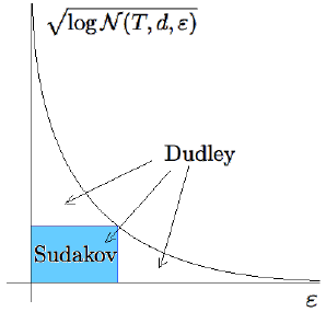
8.1 Dudley’s inequality 191
Figure 8.1 Dudley’s inequality bounds E sup
t∈T
X
t
by the area under the
curve. Sudakov’s inequality bounds it below by the largest area of a
rectangle under the curve, up to constants.
Our proof of this theorem will be based on the important technique of chaining,
which can be useful in many other problems. Chaining is a multi-scale version
of the ε-net argument that we used successfully in the past, for example in the
proofs of Theorems 4.4.5 and 7.7.1.
In the familiar, single-scale ε-net argument, we discretize T by choosing an
ε-net N of T . Then every point t ∈ T can be approximated by a closest point
from the net π(t) ∈ N with accuracy ε, so that d(t, π(t)) ≤ ε. The increment
condition (8.1) yields
∥X
t
− X
π(t)
∥
ψ
2
≤ Kε. (8.3)
This gives
E sup
t∈T
X
t
≤ E sup
t∈T
X
π(t)
+ E sup
t∈T
(X
t
− X
π(t)
).
The first term can be controlled by a union bound over |N| = N(T, d, ε) points
π(t).
To bound the second term, we would like to use (8.3). But it only holds for fixed
t ∈ T , and it is not clear how to control the supremum over t ∈ T . To overcome
this difficulty, we do not stop here but continue to run the ε-net argument further,
building progressively finer approximations π
1
(t), π
2
(t), . . . to t with finer nets.
Let us now develop formally this technique of chaining.
Proof of Theorem 8.1.4. Step 1: Chaining set-up. Without loss of generality,
we may assume that K = 1 and that T is finite. (Why?) Let us set the dyadic
scale
ε
k
= 2
−k
, k ∈ Z (8.4)
and choose ε
k
-nets T
k
of T so that
|T
k
| = N(T, d, ε
k
). (8.5)

192 Chaining
Only a part of the dyadic scale will be needed. Indeed, since T is finite, there
exists a small enough number κ ∈ Z (defining the coarsest net) and a large enough
number K ∈ Z (defining the finest net), such that
T
κ
= {t
0
} for some t
0
∈ T, T
K
= T. (8.6)
For a point t ∈ T , let π
k
(t) denote a closest point in T
k
, so we have
d(t, π
k
(t)) ≤ ε
k
. (8.7)
Since E X
t
0
= 0, we have
E sup
t∈T
X
t
= E sup
t∈T
(X
t
− X
t
0
).
We can express X
t
− X
t
0
as a telescoping sum; think about walking from t
0
to t
along a chain of points π
k
(t) that mark progressively finer approximations to t:
X
t
− X
t
0
= (X
π
κ
(t)
− X
t
0
) + (X
π
κ+1
(t)
− X
π
κ
(t)
) + ··· + (X
t
− X
π
K
(t)
), (8.8)
see Figure 8.2 for illustration. The first and last terms of this sum are zero by
Figure 8.2 Chaining: a walk from a fixed point t
0
to an arbitrary point t in
T along elements π
k
(T ) of progressively finer nets of T
(8.6), so we have
X
t
− X
t
0
=
K
X
k=κ+1
(X
π
k
(t)
− X
π
k−1
(t)
). (8.9)
Since the supremum of the sum is bounded by the sum of suprema, this yields
E sup
t∈T
(X
t
− X
t
0
) ≤
K
X
k=κ+1
E sup
t∈T
(X
π
k
(t)
− X
π
k−1
(t)
). (8.10)
Step 2: Controlling the increments. Although each term in the bound
(8.10) still has a supremum over the entire set T , a closer look reveals that it is
actually a maximum over a much smaller set, namely the set all possible pairs
(π
k
(t), π
k−1
(t)). The number of such pairs is
|T
k
| · |T
k−1
| ≤ |T
k
|
2
,

8.1 Dudley’s inequality 193
a number that we can control through (8.5).
Next, for a fixed t, the increments in (8.10) can be bounded as follows:
∥X
π
k
(t)
− X
π
k−1
(t)
∥
ψ
2
≤ d(π
k
(t), π
k−1
(t)) (by (8.1) and since K = 1)
≤ d(π
k
(t), t) + d(t, π
k−1
(t)) (by triangle inequality)
≤ ε
k
+ ε
k−1
(by (8.7))
≤ 2ε
k−1
.
Recall from Exercise 2.5.10 that the expected maximum of N sub-gaussian
random variables is at most CL
√
log N where L is the maximal ψ
2
norm. Thus
we can bound each term in (8.10) as follows:
E sup
t∈T
(X
π
k
(t)
− X
π
k−1
(t)
) ≤ Cε
k−1
q
log |T
k
|. (8.11)
Step 3: Summing up the increments. We have shown that
E sup
t∈T
(X
t
− X
t
0
) ≤ C
K
X
k=κ+1
ε
k−1
q
log |T
k
|. (8.12)
It remains substitute the values ε
k
= 2
−k
from (8.4) and the bounds (8.5) on |T
k
|,
and conclude that
E sup
t∈T
(X
t
− X
t
0
) ≤ C
1
K
X
k=κ+1
2
−k
q
log N(T, d, 2
−k
).
Theorem 8.1.4 is proved.
Let us now deduce the integral form of Dudley’s inequality.
Proof of Dudley’s integral inequality, Theorem 8.1.3. To convert the sum (8.2)
into an integral, we express 2
−k
as 2
R
2
−k
2
−k−1
dε. Then
X
k∈Z
2
−k
q
log N(T, d, 2
−k
) = 2
X
k∈Z
Z
2
−k
2
−k−1
q
log N(T, d, 2
−k
) dε.
Within the limits of integral, 2
−k
≥ ε, so log N(T, d, 2
−k
) ≤ log N(T, d, ε) and
the sum is bounded by
2
X
k∈Z
Z
2
−k
2
−k−1
q
log N(T, d, ε) dε = 2
Z
∞
0
q
log N(T, d, ε) dε.
The proof is complete.
Remark 8.1.5 (Supremum of increments). A quick glance at the proof reveals
that the chaining method actually yields the bound
E sup
t∈T
|X
t
− X
t
0
| ≤ CK
Z
∞
0
q
log N(T, d, ε) dε

194 Chaining
for any fixed t
0
∈ T . Combining it with a similar bound for X
s
− X
t
0
and using
triangle inequality, we deduce that
E sup
t,s∈T
|X
t
− X
s
| ≤ CK
Z
∞
0
q
log N(T, d, ε) dε.
Note that in either of these two bounds, we need not require the mean zero as-
sumption E X
t
= 0. It is required, however, in Dudley’s Theorem 8.1.3; otherwise
it may fail. (Why?)
Dudley’s inequality gives a bound on the expectation only, but adapting the
argument yields a nice tail bound as well.
Theorem 8.1.6 (Dudley’s integral inequality: tail bound). Let (X
t
)
t∈T
be a
random process on a metric space (T, d) with sub-gaussian increments as in (8.1).
Then, for every u ≥ 0, the event
sup
t,s∈T
|X
t
− X
s
| ≤ CK
Z
∞
0
q
log N(T, d, ε) dε + u · diam(T )
holds with probability at least 1 − 2 exp(−u
2
).
Exercise 8.1.7. KKK Prove Theorem 8.1.6. To this end, first obtain a high-
probability version of (8.11):
sup
t∈T
(X
π
k
(t)
− X
π
k−1
(t)
) ≤ Cε
k−1
q
log |T
k
| + z
with probability at least 1 − 2 exp(−z
2
).
Use this inequality with z = z
k
to control all such terms simultaneously. Sum-
ming them up, deduce a bound on sup
t∈T
|X
t
− X
t
0
| with probability at least
1 −2
P
k
exp(−z
2
k
). Finally, choose the values for z
k
that give you a good bound;
one can set z
k
= u +
√
k − κ for example.
Exercise 8.1.8 (Equivalence of Dudley’s integral and sum). KK In the proof
of Theorem 8.1.3 we bounded Dudley’s sum by the integral. Show the reverse
bound:
Z
∞
0
q
log N(T, d, ε) dε ≤ C
X
k∈Z
2
−k
q
log N(T, d, 2
−k
).
8.1.1 Remarks and Examples
Remark 8.1.9 (Limits of Dudley’s integral). Although Dudley’s integral is for-
mally over [0, ∞], we can clearly make the upper bound equal the diameter of T
in the metric d, thus
E sup
t∈T
X
t
≤ CK
Z
diam(T )
0
q
log N(T, d, ε) dε. (8.13)
Indeed, if ε > diam(T ) then a single point (any point in T ) is an ε-net of T ,
which shows that log N(T, d, ε) = 0 for such ε.

8.1 Dudley’s inequality 195
Let us apply Dudley’s inequality for the canonical Gaussian process, just like
we did with Sudakov’s inequality in Section 7.4.1. We immediately obtain the
following bound.
Theorem 8.1.10 (Dudley’s inequality for sets in R
n
). For any set T ⊂ R
n
, we
have
w(T) ≤ C
Z
∞
0
q
log N(T, ε) dε.
Example 8.1.11. Let us test Dudley’s inequality for the unit Euclidean ball
T = B
n
2
. Recall from (4.10) that
N(B
n
2
, ε) ≤
3
ε
n
for ε ∈ (0, 1]
and N(B
n
2
, ε) = 1 for ε > 1. Then Dudley’s inequality yields a converging integral
w(B
n
2
) ≤ C
Z
1
0
r
n log
3
ε
dε ≤ C
1
√
n.
This is optimal: indeed, as we know from (7.16), the Gaussian width of B
n
2
is
equivalent to
√
n up to a constant factor.
Exercise 8.1.12 (Dudley’s inequality can be loose). KKK Let e
1
, . . . , e
n
de-
note the canonical basis vectors in R
n
. Consider the set
T
:
=
e
k
√
1 + log k
, k = 1, . . . , n
.
(a) Show that
w(T) ≤ C,
where as usual C denotes an absolute constant.
Hint: This should be straightforward from Exercise 2.5.10.
(b) Show that
Z
∞
0
q
log N(T, d, ε) dε → ∞
as n → ∞.
Hint: The first m vectors in T form a (1/
√
log m)-separated set.
8.1.2 * Two-sided Sudakov’s inequality
This sub-section is optional; further material is not based on it.
As we just saw in Exercise 8.1.12, in general there is a gap between Sudakov’s
and Dudley’s inequalities. Fortunately, this gap is only logarithmically large. Let
us make this statement more precise and show that Sudakov’s inequality in R
n
(Corollary 7.4.3) is optimal up to a log n factor.

196 Chaining
Theorem 8.1.13 (Two-sided Sudakov’s inequality). Let T ⊂ R
n
and set
s(T )
:
= sup
ε≥0
ε
q
log N(T, ε).
Then
c · s(T ) ≤ w(T ) ≤ C log(n) · s(T ).
Proof The lower bound is a form of Sudakov’s inequality (Corollary 7.4.3). To
prove the upper bound, the main idea is that the chaining process converges
exponentially fast, and thus O(log n) steps should suffice to walk from t
0
to
somewhere very near t.
As we already noted in (8.13), the coarsest scale in the chaining sum (8.9) can
be chosen as the diameter of T . In other words, we can start the chaining at κ
which is the smallest integer such that
2
−κ
< diam(T ).
This is not different from what we did before. What will be different is the finest
scale. Instead of going all the way down, let us stop chaining at K which is the
largest integer for which
2
−K
≥
w(T)
4
√
n
.
(It will be clear why we made this choice in a second.)
Then the last term in (8.8) may not be zero as before, and instead of (8.9) we
need to bound
w(T) ≤
K
X
k=κ+1
E sup
t∈T
(X
π
k
(t)
− X
π
k−1
(t)
) + E sup
t∈T
(X
t
− X
π
K
(t)
). (8.14)
To control the last term, recall that X
t
= ⟨g, t⟩ is the canonical process, so
E sup
t∈T
(X
t
− X
π
K
(t)
) = E sup
t∈T
g, t − π
K
(t)
≤ 2
−K
· E ∥g∥
2
(since ∥t − π
K
(t)∥
2
≤ 2
−K
)
≤ 2
−K
√
n
≤
w(T)
2
√
n
·
√
n (by definition of K)
≤
1
2
w(T).
Putting this into (8.14) and subtracting
1
2
w(T) from both sides, we conclude that
w(T) ≤ 2
K
X
k=κ+1
E sup
t∈T
(X
π
k
(t)
− X
π
k−1
(t)
). (8.15)
Thus, we have removed the last term from (8.14). Each of the remaining terms

8.2 Application: empirical processes 197
can be bounded as before. The number of terms in this sum is
K − κ ≤ log
2
diam(T )
w(T)/4
√
n
(by definition of K and κ)
≤ log
2
4
√
n ·
√
2π
(by property f of Proposition 7.5.2)
≤ C log n.
Thus we can replace the sum by the maximum in (8.15) by paying a factor C log n.
This completes the argument like before, in the proof of Theorem 8.1.4.
Exercise 8.1.14 (Limits in Dudley’s integral). KKK Prove the following im-
provement of Dudley’s inequality (Theorem 8.1.10). For any set T ⊂ R
n
, we
have
w(T) ≤ C
Z
b
a
q
log N(T, ε) dε where a =
cw(T)
√
n
, b = diam(T ).
8.2 Application: empirical processes
We give an application of Dudley’s inequality to empirical processes, which are
certain random processes indexed by functions. The theory of empirical processes
is a large branch of probability theory, and we only scratch its surface here. Let
us consider a motivating example.
8.2.1 Monte-Carlo method
Suppose we want to evaluate the integral of a function f
:
Ω → R with respect
to some probability measure µ on some domain Ω ⊂ R
d
:
Z
Ω
f dµ,
see Figure 8.3a. For example, we could be interested in computing
R
1
0
f(x) dx for
a function f
:
[0, 1] → R.
We use probability to evaluate this integral. Consider a random point X that
takes values in Ω according to the law µ, i.e.
P
X ∈ A
= µ(A) for any measurable set A ⊂ Ω.
(For example, to evaluate
R
1
0
f(x) dx, we take X ∼ Unif[0, 1].) Then we may
interpret the integral as expectation:
Z
Ω
f dµ = E f(X).
Let X
1
, X
2
, . . . be i.i.d. copies of X. The law of large numbers (Theorem 1.3.1)
yields that
1
n
n
X
i=1
f(X
i
) → E f(X) almost surely (8.16)

198 Chaining
(a) The problem is to compute the
integral of f on a domain Ω.
(b) The integral is approximated by the
sum
1
n
P
n
1
f(X
i
) with randomly sampled
points X
i
.
Figure 8.3 Monte-Carlo method for randomized, numerical integration.
as n → ∞. This means that we can approximate the integral by the sum
Z
Ω
f dµ ≈
1
n
n
X
i=1
f(X
i
) (8.17)
where the points X
i
are drawn at random from the domain Ω; see Figure 8.3b
for illustration. This way of numerically computing integrals is called the Monte-
Carlo method.
Remark 8.2.1 (Error rate). Note that the average error in (8.17) is O(1/
√
n).
Indeed, as we note in (1.5), the rate of convergence in the law of large numbers
is
E
1
n
n
X
i=1
f(X
i
) − E f(X)
≤
Var
1
n
n
X
i=1
f(X
i
)
1/2
= O
1
√
n
. (8.18)
Remark 8.2.2. Note that we do not even need to know the measure µ to evaluate
the integral
R
Ω
f dµ; it suffices to be able to draw random samples X
i
according
to µ. Similarly, we do not even need to know f at all points in the domain; a few
random points suffice.
8.2.2 A uniform law of large numbers
Can we use the same sample X
1
, . . . , X
n
to evaluate the integral of any function
f
:
Ω → R? Of course, not. For a given sample, one can choose a function that
oscillates in a the wrong way between the sample points, and the approximation
(8.17) will fail.
Will it help if we consider only those functions f that do not oscillate wildly
– for example, Lipschitz functions? It will. Our next theorem states that Monte-
Carlo method (8.17) does work well simultaneously over the class of Lipschitz
functions
F
:
=
f
:
[0, 1] → R, ∥f∥
Lip
≤ L
, (8.19)
where L is any fixed number.
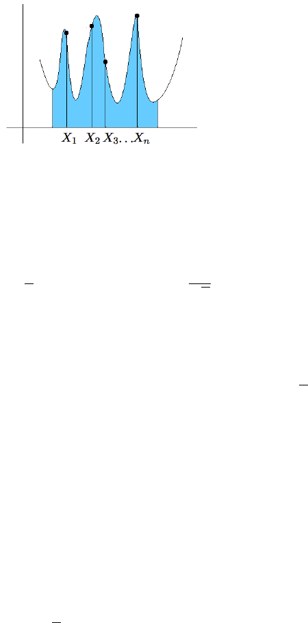
8.2 Application: empirical processes 199
Figure 8.4 One can not use the same sample X
1
, . . . , X
n
to approximate
the integral of any function f.
Theorem 8.2.3 (Uniform law of large numbers). Let X, X
1
, X
2
, . . . , X
n
be i.i.d.
random variables taking values in [0, 1]. Then
E sup
f∈F
1
n
n
X
i=1
f(X
i
) − E f(X)
≤
CL
√
n
. (8.20)
Remark 8.2.4. Before we prove this result, let us pause to emphasize its key
point: the supremum over f ∈ F appears inside the expectation. By Markov’s
inequality, this means that with high probability, a random sample X
1
, . . . , X
n
is
good. And “good” means that using this sample, we can approximate the integral
of any function f ∈ F with error bounded by the same quantity CL/
√
n. This is
the same rate of convergence the classical Law of Large numbers (8.18) guarantees
for a single function f. So we paid essentially nothing for making the law of large
numbers uniform over the class of functions F.
To prepare for the proof of Theorem 8.2.3, it will be useful to view the left
side of (8.20) as the magnitude of a random process indexed by functions f ∈ F.
Such random processes are called empirical processes.
Definition 8.2.5. Let F be a class of real-valued functions f
:
Ω → R where
(Ω, Σ, µ) is a probability space. Let X be a random point in Ω distributed ac-
cording to the law µ, and let X
1
, X
2
, . . . , X
n
be independent copies of X. The
random process (X
f
)
f∈F
defined by
X
f
:
=
1
n
n
X
i=1
f(X
i
) − E f(X) (8.21)
is called an empirical process indexed by F.
Proof of Theorem 8.2.3 Without loss of generality, it is enough to prove the
theorem for the class
F
:
=
f
:
[0, 1] → [0, 1], ∥f∥
Lip
≤ 1
. (8.22)
(Why?) We would like to bound the magnitude
E sup
f∈F
|X
f
|

200 Chaining
of the empirical process (X
f
)
f∈F
defined in (8.21).
Step 1: checking sub-gaussian increments. We can do this using Dudley’s
inequality, Theorem 8.1.3. To apply this result, we just need to check that the
empirical process has sub-gaussian increments. So, fix a pair of functions f, g ∈ F
and consider
∥X
f
− X
g
∥
ψ
2
=
1
n
n
X
i=1
Z
i
ψ
2
where Z
i
:
= (f − g)(X
i
) − E(f − g)(X).
Random variables Z
i
are independent and have mean zero. So, by Proposi-
tion 2.6.1 we have
∥X
f
− X
g
∥
ψ
2
≲
1
n
n
X
i=1
∥Z
i
∥
2
ψ
2
1/2
.
Now, using centering (Lemma 2.6.8) we have
∥Z
i
∥
ψ
2
≲ ∥(f − g)(X
i
)∥
ψ
2
≲ ∥f − g∥
∞
.
It follows that
∥X
f
− X
g
∥
ψ
2
≲
1
n
· n
1/2
∥f − g∥
∞
=
1
√
n
∥f − g∥
∞
.
Step 2: applying Dudley’s inequality. We found that the empirical process
(X
f
)
f∈F
has sub-gaussian increments with respect to the L
∞
norm. This allows
us to apply Dudley’s inequality. Note that (8.22) implies that the diameter of F
in L
∞
metric is bounded by 1. Thus
E sup
f∈F
|X
f
| = E sup
f∈F
|X
f
− X
0
| ≲
1
√
n
Z
1
0
q
log N(F, ∥ · ∥
∞
, ε) dε.
(Here we used that the zero function belongs to F and used the version of Dudley’s
inequality from Remark 8.1.5; see also (8.13)).
Using that all functions in f ∈ F are Lipschitz with ∥f∥
Lip
≤ 1, it is not
difficult to bound the covering numbers of F as follows:
N(F, ∥ · ∥
∞
, ε) ≤
C
ε
C/ε
;
we will show this in Exercise 8.2.6 below. This bound makes Dudley’s integral
converge, and we conclude that
E sup
f∈F
|X
f
| ≲
1
√
n
Z
1
0
r
C
ε
log
C
ε
dε ≲
1
√
n
.
Theorem 8.2.3 is proved.
Exercise 8.2.6 (Metric entropy of the class of Lipschitz functions). KKK Con-
sider the class of functions
F
:
=
f
:
[0, 1] → [0, 1], ∥f∥
Lip
≤ 1
.

8.2 Application: empirical processes 201
Show that
N(F, ∥ ·∥
∞
, ε) ≤
2
ε
2/ε
for any ε ∈ (0, 1).
Hint: Put a mesh on the square [0, 1]
2
with step ε. Given f ∈ F, show that ∥f − f
0
∥
∞
≤ ε for some
function f
0
whose graph follows the mesh; see Figure 8.5. The number all mesh-following functions f
0
is bounded by (1/ε)
1/ε
. Next, use the result of Exercise 4.2.9.
Figure 8.5 Bounding the metric entropy of the class of Lipschitz functions
in Exercise 8.2.6. A Lipschitz function f is approximated by a function f
0
on
a mesh.
Exercise 8.2.7 (An improved bound on the metric entropy). KKK Improve
the bound in Exercise 8.2.6 to
N(F, ∥ ·∥
∞
, ε) ≤ e
C/ε
for any ε > 0.
Hint: Use that f is Lipschitz to find a better bound on the number of possible functions f
0
.
Exercise 8.2.8 (Higher dimensions). KKK Let [0, 1]
d
be the unit cube in di-
mension d ≥ 1 equipped with the ∥·∥
∞
metric. Consider the class of functions
F
:
=
n
f
:
[0, 1]
d
→ R, f(0) = 0, ∥f∥
Lip
≤ 1
o
.
Show that
N(F, ∥ · ∥
∞
, ε) ≤ e
C/ε
d
for any ε > 0.
8.2.3 Empirical measure
Let us take one more look at the Definition 8.2.5 of empirical processes. Consider
a probability measure µ
n
that is uniformly distributed on the sample X
1
, . . . , X
n
,
that is
µ
n
({X
i
}) =
1
n
for every i = 1, . . . , n. (8.23)
Note that µ
n
is a random measure. It is called the empirical measure.
While the integral of f with respect to the original measure µ is the E f(X) (the
“population” average of f ) the integral of f with respect to the empirical measure

202 Chaining
is
1
n
P
n
i=1
f(X
i
) (the “sample”, or empirical, average of f). In the literature on
empirical processes, the population expectation of f is denoted by µf, and the
empirical expectation, by µ
n
f:
µf =
Z
f dµ = E f(X), µ
n
f =
Z
f dµ
n
=
1
n
n
X
i=1
f(X
i
).
The empirical process X
f
in (8.21) thus measures the deviation of population
expectation from the empirical expectation:
X
f
= µf − µ
n
f.
The uniform law of large numbers (8.20) gives a uniform bound on the deviation
E sup
f∈F
|µ
n
f − µf| (8.24)
over the class of Lipschitz functions F defined in (8.19).
The quantity (8.24) can be thought as a distance between the measures µ
n
and
µ. It is called the Wasserstein’s distance W
1
(µ, µ
n
) . The Wasserstein distance has
an equivalent formulation as the transportation cost of measure µ into measure
µ
n
, where the cost of moving a mass (probability) p > 0 is proportional to p
and to the distance moved. The equivalence between the transportation cost and
(8.24) is provided by Kantorovich-Rubinstein’s duality theorem.
8.3 VC dimension
In this section, we introduce the notion of VC dimension, which plays a major
role in statistical learning theory. We relate VC dimension to covering numbers,
and then, through Dudley’s inequality, to random processes and uniform law of
large numbers. Applications to statistical learning theory will be given in next
section.
8.3.1 Definition and examples
VC-dimension is a measure of complexity of classes of Boolean functions. By a
class of Boolean functions we mean any collection F of functions f
:
Ω → {0, 1}
defined on a common domain Ω.
Definition 8.3.1 (VC dimension). Consider a class F of Boolean functions on
some domain Ω. We say that a subset Λ ⊆ Ω is shattered by F if any function
g
:
Λ → {0, 1} can be obtained by restricting some function f ∈ F onto Λ. The
VC dimension of F, denoted vc(F), is the largest cardinality
1
of a subset Λ ⊆ Ω
shattered by F.
The definition of VC dimension may take some time to fully comprehend. We
work out a few examples to illustrate this notion.
1
If the largest cardinality does not exist, we set vc(F) = ∞.

8.3 VC dimension 203
Example 8.3.2 (Intervals). Let F be the class of indicators of all closed intervals
in R, that is
F
:
=
1
[a,b]
:
a, b ∈ R, a ≤ b
.
We claim that there exists a two-point set Λ ⊂ R that is shattered by F, and
thus
vc(F) ≥ 2.
Take, for example, Λ
:
= {3, 5}. It is easy to see that each of the four possible
functions g
:
Λ → {0, 1} is a restriction of some indicator function f = 1
[a,b]
onto
Λ. For example, the function g defined by g(3) = 1, g(5) = 0 is a restriction of
f = 1
[2,4]
onto Λ, since f(3) = g(3) = 1 and f(5) = g(5) = 0. The three other
possible functions g can be treated similarly; see Figure 8.6. Thus Λ = {3, 5} is
indeed shattered by F, as claimed.
Figure 8.6 The function g(3) = g(5) = 0 is a restriction of 1
[6,7]
onto
Λ = {3, 5} (left). The function g(3) = 0, g(5) = 1 is a restriction of 1
[4,6]
onto Λ (middle left). The function g(3) = 1, g(5) = 0 is a restriction of 1
[2,4]
onto Λ (middle right). The function g(3) = g(5) = 1 is a restriction of 1
[2,6]
onto Λ (right).
Next, we claim that no three-point set Λ = {p, q, r} can be shattered by F,
and thus
vc(F) = 2.
To see this, assume p < q < r and define the function g
:
Λ → {0, 1} by g(p) = 1,
g(q) = 0, g(r) = 1. Then g can not be a restriction of any indicator 1
[a,b]
onto Λ,
for otherwise [a, b] must contain two points p and r but not the point q that lies
between them, which is impossible.
Example 8.3.3 (Half-planes). Let F be the class of indicators of all closed half-
planes in R
2
. We claim that there is a three-point set Λ ⊂ R
2
that is shattered
by F, and thus
vc(F) ≥ 3.
To see this, let Λ be a set of three points in general position, such as in Figure 8.7.
Then each of the 2
3
= 8 functions g
:
Λ → {0, 1} is a restriction of the indicator
function of some half-plane. To see this, arrange the half-plane to contain exactly
those points of Λ where g takes value 1, which can always be done – see Figure 8.7.

204 Chaining
Figure 8.7 Left: a three-point set Λ and function g
:
Λ → {0, 1} (values
shown in blue). Such g is a restriction of the indicator function of the shaded
half-plane. Middle and right: two kinds of four-points sets Λ in general
position, and functions g
:
Λ → {0, 1}. In each case, no half-plane can
contain exactly the points with value 1. Thus, g is not a restriction of the
indicator function of any half-plane.
Next, we claim that no four-point set can be shattered by F, and thus
vc(F) = 3.
There are two possible arrangements of the four-point sets Λ in general position,
shown in Figure 8.7. (What if Λ is not in general position? Analyze this case.) In
each of the two cases, there exists a 0/1 labeling of the points 0 and 1 such that
no half-plane can contain exactly the points labeled 1; see Figure 8.7. This means
that in each case, there exists a function g
:
Λ → {0, 1} that is not a restriction
of any function f ∈ F onto Λ, and thus Λ is not shattered by F as claimed.
Example 8.3.4. Let Ω = {1, 2, 3}. We can conveniently represent Boolean func-
tions on Ω as binary strings of length three. Consider the class
F
:
= {001, 010, 100, 111}.
The set Λ = {1, 3} is shattered by F. Indeed, restricting the functions in F onto Λ
amounts to dropping the second digit, thus producing strings 00, 01, 10, 11. Thus,
the restriction produces all possible binary strings of length two, or equivalently,
all possible functions g
:
Λ → {0, 1}. Hence Λ is shattered by F, and thus
vc(F) ≥ |Λ| = 2. On the other hand, the (only) three-point set {1, 2, 3} is not
shattered by F, as this would require all eight binary digits of length three to
appear in F, which is not true.
Exercise 8.3.5 (Pairs of intervals). KK Let F be the class of indicators of sets
of the form [a, b] ∪ [c, d] in R. Show that
vc(F) = 4.
Exercise 8.3.6 (Circles). KKK Let F be the class of indicators of all circles
in R
2
. Show that
vc(F) = 3.
Exercise 8.3.7 (Rectangles). KKK Let F be the class of indicators of all
8.3 VC dimension 205
closed axis-aligned rectangles, i.e. product sets [a, b] × [c, d], in R
2
. Show that
vc(F) = 4.
Exercise 8.3.8 (Squares). KKK Let F be the class of indicators of all closed
axis-aligned squares, i.e. product sets [a, a + d] × [b, b + d], in R
2
. Show that
vc(F) = 3.
Exercise 8.3.9 (Polygons). KKK Let F be the class of indicators of all convex
polygons in R
2
, without any restriction on the number of vertices. Show that
vc(F) = ∞.
Remark 8.3.10 (VC dimension of classes of sets). We may talk about VC di-
mension of classes of sets instead of functions. This is due to the natural corre-
spondence between the two: a Boolean function f on Ω determines the subset
{x ∈ Ω
:
f(x) = 1}, and, vice versa, a subset Ω
0
⊂ Ω determines the Boolean
function f = 1
Ω
0
. In this language, the VC dimension of the set of intervals in R
equals 2, the VC dimension of the set of half-planes in R
2
equals 3, and so on.
Exercise 8.3.11. K Give the definition of VC dimension of a class of subsets
of Ω without mentioning any functions.
Remark 8.3.12 (More examples). It can be shown that the VC dimension of
the class of all rectangles on the plane (not necessarily axis-aligned) equals 7. For
the class of all polygons with k vertices on the plane, the VC dimension is also
2k + 1. For the class of half-spaces in R
n
, the VC dimension is n + 1.
8.3.2 Pajor’s Lemma
Consider a class of Boolean functions F on a finite set Ω. We study a remark-
able connection between the cardinality |F| and VC dimension of F. Somewhat
oversimplifying, we can say that |F| is exponential in vc(F). A lower bound is
trivial:
|F| ≥ 2
vc(F)
.
(Check!) We now pass to upper bounds; they are less trivial. The following lemma
states that there are as many shattered subsets of Ω as the functions in F.
Lemma 8.3.13 (Pajor’s Lemma). Let F be a class of Boolean functions on a
finite set Ω. Then
|F| ≤
n
Λ ⊆ Ω
:
Λ is shattered by F
o
.
We include the empty set Λ = ∅ in the counting on the right side.
Before we prove Pajor’s lemma, let us pause to give a quick illustration using
Example 8.3.4. There |F| = 4 and there are six subsets Λ that are shattered by
F, namely {1}, {2}, {3}, {1, 2}, {1, 3} and {2, 3}. (Check!) Thus the inequality
in Pajor’s lemma reads 4 ≤ 6 in this case.

206 Chaining
Proof of Pajor’s Lemma 8.3.13. We proceed by induction on the cardinality of
Ω. The case |Ω| = 1 is trivial, since we include the empty set in the counting.
Assume the lemma holds for any n-point set Ω, and let us prove it for Ω with
|Ω| = n + 1.
Chopping out one (arbitrary) point from the set Ω, we can express it as
Ω = Ω
0
∪ {x
0
}, where |Ω
0
| = n.
The class F then naturally breaks into two sub-classes
F
0
:
= {f ∈ F
:
f(x
0
) = 0} and F
1
:
= {f ∈ F
:
f(x
0
) = 1}.
By the induction hypothesis, the counting function
S(F) =
n
Λ ⊆ Ω
:
Λ is shattered by F
o
satisfies
2
S(F
0
) ≥ |F
0
| and S(F
1
) ≥ |F
1
|. (8.25)
To complete the proof, all we need to check is
S(F) ≥ S(F
0
) + S(F
1
), (8.26)
for then (8.25) would give S(F) ≥ |F
0
| + |F
1
| = |F|, as needed.
Inequality (8.26) may seem trivial. Any set Λ that is shattered by F
0
or F
1
is
automatically shattered by the larger class F, and thus each set Λ counted by
S(F
0
) or S(F
1
) is automatically counted by S(F). The problem, however, lies
in the double counting. Assume the same set Λ is shattered by both F
0
and F
1
.
The counting function S(F) will not count Λ twice. However, a different set will
be counted by S(F), which was not counted by either S(F
0
) or S(F
1
) – namely,
Λ ∪ {x
0
}. A moment’s thought reveals that this set is indeed shattered by F.
(Check!) This establishes inequality (8.26) and completes the proof of Pajor’s
Lemma.
It may be helpful to illustrate the key point in the proof of Pajor’s lemma with
a specific example.
Example 8.3.14. Let us again go back to Example 8.3.4. Following the proof of
Pajor’s lemma, we chop out x
0
= 3 from Ω = {1, 2, 3}, making Ω
0
= {1, 2}. The
class F = {001, 010, 100, 111} then breaks into two sub-classes
F
0
= {010, 100} and F
1
= {001, 111}.
There are exactly two subsets Λ shattered by F
0
, namely {1} and {2}, and the
same subsets are shattered by F
1
, making S(F
0
) = S(F
1
) = 2. Of course, the
same two subsets are also shattered by F, but we need two more shattered subsets
to make S(F) ≥ 4 for the key inequality (8.26). Here is how we construct them:
append x
0
= 3 to the already counted subsets Λ. The resulting sets {1, 3} and
2
To properly use the induction hypothesis here, restrict the functions in F
0
and F
1
onto the n-point
set Ω
0
.

8.3 VC dimension 207
{2, 3} are also shattered by F, and we have not counted them yet. Now have at
least four subsets shattered by F, making the key inequality (8.26) in the proof
Pajor’s lemma true.
Exercise 8.3.15 (Sharpness of Pajor’s Lemma). KK Show that Pajor’s Lemma 8.3.13
is sharp.
Hint: Consider the set F of binary strings of length n with at most d ones. This set is called Hamming
cube.
8.3.3 Sauer-Shelah Lemma
We now deduce a remarkable upper bound on the cardinality of a function class
in terms of VC dimension.
Theorem 8.3.16 (Sauer-Shelah Lemma). Let F be a class of Boolean functions
on an n-point set Ω. Then
|F| ≤
d
X
k=0
n
k
!
≤
en
d
d
where d = vc(F).
Proof Pajor’s Lemma states that |F| is bounded by the number of subsets Λ ⊆
Ω that are shattered by F. The cardinality of each such set Λ is bounded by
d = vc(F), according to the definition of VC dimension. Thus
|F| ≤
n
Λ ⊆ Ω
:
|Λ| ≤ d
o
=
d
X
k=0
n
k
!
since the sum in right hand side gives the total number of subsets of an n-element
set with cardinalities at most k. This proves the first inequality of Sauer-Shelah
Lemma. The second inequality follows from the bound on the binomial sum we
proved in Exercise 0.0.5.
Exercise 8.3.17 (Sharpness of Sauer-Shelah Lemma). KK Show that Sauer-
Shelah lemma is sharp for all n and d.
Hint: Consider Hamming cube from Exercise 8.3.15.
8.3.4 Covering numbers via VC dimension
Sauer-Shelah Lemma is sharp, but it can only be used for finite function classes
F. What about infinite function classes F, for example the indicator functions of
half-planes in Example 8.3.3? It turns out that we can always bound the covering
numbers of F in terms of VC dimension.
Let F be a class of Boolean functions on a set Ω as before, and let µ be any
probability measure on Ω. Then F can be considered as a metric space under the

208 Chaining
L
2
(µ) norm, with the metric on F given by
d(f, g) = ∥f − g∥
L
2
(µ)
=
Z
Ω
|f − g|
2
dµ
1/2
, f, g ∈ F.
Then we can talk about covering numbers of the class F in the L
2
(µ) norm, which
we denote
3
N(F, L
2
(µ), ε).
Theorem 8.3.18 (Covering numbers via VC dimension). Let F be a class of
Boolean functions on a probability space (Ω, Σ, µ). Then, for every ε ∈ (0, 1), we
have
N(F, L
2
(µ), ε) ≤
2
ε
Cd
where d = vc(F).
This result should be compared to the volumetric bound (4.10), which also
states that the covering numbers scale exponentially with the dimension. The
important difference is that the VC dimension captures a combinatorial rather
than linear algebraic complexity of sets.
For a first attempt at proving Theorem 8.3.18, let us assume for a moment
that Ω is finite, say |Ω| = n. Then Sauer-Shelah Lemma (Theorem 8.3.16) yields
N(F, L
2
(µ), ε) ≤ |F| ≤
en
d
d
.
This is not quite what Theorem 8.3.18 claims, but it comes close. To improve the
bound, we need to remove the dependence on the size n of Ω. Can we reduce the
domain Ω to a much smaller subset without harming the covering numbers? It
turns out that we can; this will be based on the following lemma.
Lemma 8.3.19 (Dimension reduction). Let F be a class of N Boolean functions
on a probability space (Ω, Σ, µ). Assume that all functions in F are ε-separated,
that is
∥f − g∥
L
2
(µ)
> ε for all distinct f, g ∈ F.
Then there exist a number n ≤ Cε
−4
log N and an n-point set Ω
n
⊂ Ω such that
the restrictions of the functions f ∈ F onto Ω
n
are all distinct.
Proof Our argument will be based on the probabilistic method. We choose the
subset Ω
n
at random and show that it satisfies the conclusion of the theorem
with positive probability. This will automatically imply the existence of at least
one suitable choice of Ω
n
.
3
If you are not completely comfortable with measure theory, it may be helpful to consider a discrete
case, which is all we need for applications in the next section. Let Ω be an N-point set, say
Ω = {1, . . . , N} and µ be the uniform measure on Ω, thus µ(i) = 1/N for every i = 1, . . . , N . In this
case, the L
2
(µ) norm of a function f
:
Ω → R is simply ∥f∥
L
2
(µ)
= (
1
N
P
N
i=1
f(i)
2
)
1/2
.
Equivalently, one can think of f as a vector in R
N
. The L
2
(µ) is just the scaled Euclidean norm
∥ · ∥
2
on R
n
, i.e. ∥f∥
L
2
(µ)
= (1/
√
N)∥f∥
2
.

8.3 VC dimension 209
Let X, X
1
, . . . , X
n
independent be random points in Ω distributed
4
according
to the law µ. Define the empirical probability measure µ
n
on Ω by assigning each
point X
i
probability 1/n, allowing multiplicities. We would like to show that with
positive probability the following event holds:
∥f − g∥
2
L
2
(µ
n
)
:
=
1
n
n
X
i=1
(f − g)(X
i
)
2
> 0 for all distinctf, g ∈ F.
This would guarantee that the restrictions of the functions f ∈ F onto Ω
n
:
=
{X
1
, . . . , X
n
} are all distinct.
5
Fix a pair of distinct functions f, g ∈ F and denote h
:
= (f − g)
2
for conve-
nience. We would like to bound the deviation
∥f − g∥
2
L
2
(µ
n
)
− ∥f − g∥
2
L
2
(µ)
=
1
n
n
X
i=1
h(X
i
) − E h(X).
We have a sum of independent random variables on the right, and we use general
Hoeffding’s inequality to bound it. To do this, we first check that these random
variables are subgaussian. Indeed,
6
∥h(X
i
) − E h(X)∥
ψ
2
≲ ∥h(X)∥
ψ
2
(by Centering Lemma 2.6.8)
≲ ∥h(X)∥
∞
(by (2.17))
≤ 1 (since h = f − g with f, g Boolean).
Then general Hoeffding’s inequality (Theorem 2.6.2) gives
P
(
∥f − g∥
2
L
2
(µ
n
)
− ∥f − g∥
2
L
2
(µ)
>
ε
2
4
)
≤ 2 exp(−cnε
4
).
(Check!) Therefore, with probability at least 1 − 2 exp(−cnε
4
), we have
∥f − g∥
2
L
2
(µ
n
)
≥ ∥f − g∥
2
L
2
(µ)
−
ε
2
4
≥ ε
2
−
ε
2
4
=
3ε
2
4
, (8.27)
where we used triangle inequality and the assumption of the lemma.
This is a good bound, and even stronger than we need, but we proved it for a
fixed pair f, g ∈ F so far. Let us take a union bound over all such pairs; there are
at most N
2
of them. Then, with probability at least
1 − N
2
· 2 exp(−cnε
4
), (8.28)
the lower bound (8.27) holds simultaneously for all pairs of distinct functions
f, g ∈ F. We can make (8.28) positive by choosing n
:
= ⌈C
′
ε
−4
log N⌉ with
a sufficiently large absolute constant C. Thus the random set Ω
n
satisfies the
conclusion of the lemma with positive probability.
4
For example, if Ω = {1, . . . , N} then X is a random variable which takes values 1, . . . , N with
probability 1/N each.
5
Due to possible multiplicities among the points X
i
, the random set Ω
n
may contain fewer than n
points. If this happens, we can add arbitrarily chosen points to Ω
n
to bring its cardinality to n.
6
The inequalities “≲” below hide absolute constant factors.

210 Chaining
Proof of Theorem 8.3.18 Let us choose
N ≥ N(F, L
2
(µ), ε)
ε-separated functions in F. (To see why they exist, recall the covering-packing
relationship in Lemma 4.2.8.) Apply Lemma 8.3.19 to those functions. We obtain
a subset Ω
n
⊂ Ω with
|Ω
n
| = n ≤ Cε
−4
log N
such that the restrictions of those functions onto Ω
n
are still ε/2-separated in
L
2
(µ
n
). We use a much weaker fact – that these restrictions are just distinct.
Summarizing, we have a class F
n
of distinct Boolean functions on Ω
n
, obtained
as restrictions of certain functions from F.
Apply Sauer-Shelah Lemma (Theorem 8.3.16) for F
n
. It gives
N ≤
en
d
n
d
n
≤
Cε
−4
log N
d
n
d
n
where d
n
= vc(F
n
). Simplifying this bound,
7
we conclude that
N ≤ (Cε
−4
)
2d
n
.
To complete the proof, replace d
n
= vc(F
n
) in this bound by the larger quantity
d = vc(F).
Remark 8.3.20 (Johnson-Lindenstrauss Lemma for coordinate projections).
You may spot a similarity between Dimension Reduction Lemma 8.3.19 and an-
other dimension reduction result, Johnson-Lindenstrauss Lemma (Theorem 5.3.1).
Both results state that a random projection of a set of N points onto a dimen-
sion of subspace log N preserves the geometry of the set. The difference is in the
distribution of the random subspace. In Johnson-Lindenstrauss Lemma, it is uni-
formly distributed in the Grassmanian, and in Lemma 8.3.19 it is a coordinate
subspace.
Exercise 8.3.21 (Dimension reduction for covering numbers). KK Let F be
a class of functions on a probability space (Ω, Σ, µ), which are all bounded
by 1 in absolute value. Let ε ∈ (0, 1). Show that there exists a number n ≤
Cε
−4
log N(F, L
2
(µ), ε) and an n-point subset Ω
n
⊂ Ω such that
N(F, L
2
(µ), ε) ≤ N(F, L
2
(µ
n
), ε/4)
where µ
n
denotes the uniform probability measure on Ω
n
.
Hint: Argue as in Lemma 8.3.19 and then use the covering-packing relationship from Lemma 4.2.8.
Exercise 8.3.22. KK Theorem 8.3.18 is stated for ε ∈ (0, 1). What bound
holds for larger ε?
7
To do this, note that
log N
2d
n
= log(N
1/2d
n
) ≤ N
1/2d
n
.

8.3 VC dimension 211
8.3.5 Empirical processes via VC dimension
Let us turn again to the concept of empirical processes that we first introduced
in Section 8.2.2. There we showed how to control one specific example of an
empirical process, namely the process on the class of Lipschitz functions. In this
section we develop a general bound for an arbitrary class Boolean functions.
Theorem 8.3.23 (Empirical processes via VC dimension). Let F be a class
of Boolean functions on a probability space (Ω, Σ, µ) with finite VC dimension
vc(F) ≥ 1. Let X, X
1
, X
2
, . . . , X
n
be independent random points in Ω distributed
according to the law µ. Then
E sup
f∈F
1
n
n
X
i=1
f(X
i
) − E f(X)
≤ C
r
vc(F)
n
. (8.29)
We can quickly derive this result from Dudley’s inequality combined with the
bound on the covering numbers we just proved in Section 8.3.4. To carry out
this argument, it would be helpful to preprocess the empirical process using sym-
metrization.
Exercise 8.3.24 (Symmetrization for empirical processes). KK Let F be a
class of functions on a probability space (Ω, Σ, µ). Let X, X
1
, X
2
, . . . , X
n
be ran-
dom points in Ω distributed according to the law µ. Prove that
E sup
f∈F
1
n
n
X
i=1
f(X
i
) − E f(X)
≤ 2 E sup
f∈F
1
n
n
X
i=1
ε
i
f(X
i
)
where ε
1
, ε
2
, . . . are independent symmetric Bernoulli random variables (which
are also independent of X
1
, X
2
, . . .).
Hint: Modify the proof of Symmetrization Lemma 6.4.2.
Proof of Theorem 8.3.23 First we use symmetrization and bound the left hand
side of (8.29) by
2
√
n
E sup
f∈F
|Z
f
| where Z
f
:
=
1
√
n
n
X
i=1
ε
i
f(X
i
).
Next we condition on (X
i
), leaving all randomness in the random signs (ε
i
). We
are going to use Dudley’s inequality to bound the process (Z
f
)
f∈F
. For simplicity,
let us drop the absolute values for Z
f
for a moment; we will deal with this minor
issue in Exercise 8.3.25.
To apply Dudley’s inequality, we need to check that the increments of the
process (Z
f
)
f∈F
are sub-gaussian. These are
∥Z
f
− Z
g
∥
ψ
2
=
1
√
n
n
X
i=1
ε
i
(f − g)(X
i
)
ψ
2
≲
1
n
n
X
i=1
(f − g)(X
i
)
2
1/2
.
Here we used Proposition 2.6.1 and the obvious fact that ∥ε
i
∥
ψ
2
≲ 1.
8
We can
8
Keep in mind that here X
i
and thus (f − g)(X
i
) are fixed numbers due to conditioning.

212 Chaining
interpret the last expression as the L
2
(µ
n
) norm of the function f − g, where µ
n
is the uniform probability measure supported on the subset {X
1
, . . . , X
n
} ⊂ Ω.
9
In other words, the increments satisfy
∥Z
f
− Z
g
∥
ψ
2
≲ ∥f − g∥
L
2
(µ
n
)
.
Now we can use Dudley’s inequality (Theorem 8.1.3) conditionally on (X
i
) and
get
10
2
√
n
E sup
f∈F
Z
f
≲
1
√
n
E
Z
1
0
q
log N(F, L
2
(µ
n
), ε) dε. (8.30)
The expectation in the right hand side is obviously with respect to (X
i
).
Finally, we use Theorem 8.3.18 to bound the covering numbers:
log N(F, L
2
(µ
n
), ε) ≲ vc(F) log
2
ε
.
When we substitute this into (8.30), we get the integral of
p
log(2/ε), which is
bounded by an absolute constant. This gives
2
√
n
E sup
f∈F
Z
f
≲
r
vc(F)
n
,
as required.
Exercise 8.3.25 (Reinstating absolute value). KKK In the proof above, we
bounded E sup
f∈F
Z
f
instead of E sup
f∈F
|Z
f
|. Give a bound for the latter quan-
tity.
Hint: Add the zero function to the class F and use Remark 8.1.5 to bound |Z
f
| = |Z
f
− Z
0
|. Can the
addition of one (zero) function significantly increase the VC dimension of F?
Let us examine an important application of Theorem 8.3.23, which is called
Glivenko-Cantelli Theorem. It addresses one of the most basic problems in statis-
tics: how can we estimate the distribution of a random variable by sampling? Let
X be a random variable with unknown cumulative distribution function (CDF)
F (x) = P
X ≤ x
, x ∈ R.
Suppose we have a sample X
1
, . . . , X
n
of i.i.d. random variables drawn from
the same distribution as X. Then we can hope that F (x) could be estimated
by computing the fraction of the sample points satisfying X
i
≤ x, i.e. by the
empirical distribution function
F
n
(x)
:
=
{i ∈ [n]
:
X
i
≤ x}
n
, x ∈ R.
Note that F
n
(x) is a random function.
9
Recall that we have already encountered the empirical measure µ
n
and the L
2
(µ
n
) norm a few
times before, in particular in Lemma 8.3.19 and its proof, as well as in (8.23).
10
The diameter of F gives the upper limit according to (8.13); check that the diameter is indeed
bounded by 1.

8.3 VC dimension 213
The quantitative law of large numbers gives
E |F
n
(x) − F (x)| ≤
C
√
n
for every x ∈ R.
(Check this! Recall the variance computation in Section 1.3, but do it for the
indicator random variables 1
{X
i
≤x}
instead of X
i
.)
Glivenko-Cantelli theorem is a stronger statement, which says that F
n
approx-
imates F uniformly over x ∈ R.
Theorem 8.3.26 (Glivenko-Cantelli Theorem
11
). Let X
1
, . . . , X
n
be independent
random variables with common cumulative distribution function F . Then
E ∥F
n
− F ∥
∞
= E sup
x∈R
|F
n
(x) − F (x)| ≤
C
√
n
.
Proof This result is a particular case of Theorem 8.3.23. Indeed, let Ω = R, let
F consist of the indicators of all half-bounded intervals, i.e.
F
:
=
n
1
(−∞,x]
:
x ∈ R
o
,
and let the measure µ be the distribution
12
of X
i
. As we know from Example 8.3.2,
vc(F) ≤ 2. Thus Theorem 8.3.23 immediately implies the conclusion.
Example 8.3.27 (Discrepancy). Glivenko-Cantelli theorem can be easily gener-
alized to random vectors. (Do it!) Let us give an illustration for R
2
. Draw a sample
of i.i.d. points X
1
, . . . , X
n
from the uniform distribution on the unit square [0, 1]
2
on the plane, see Figure 8.8. Consider the class F of indicators of all circles in
that square. From Exercise 8.3.6 we know that vc(F) = 3. (Why does intersecting
with the square does not affect the VC dimension?)
Apply Theorem 8.3.23. The sum
P
n
i=1
f(X
i
) is just the number of points in the
circle with indicator function f, and the expectation E f(X) is the area of that
circle. Then we can interpret the conclusion of Theorem 8.3.23 as follows. With
high probability, a random sample of points X
1
, . . . , X
n
satisfies the following:
for every circle C in the square [0, 1]
2
,
number of points in C = Area(C) · n + O(
√
n).
This is an example of a result in geometric discrepancy theory. The same result
holds not only for circles but for half-planes, rectangles, squares, triangles, and
polygons with O(1) vertices, and any other class with bounded VC dimension.
11
The classical statement of Glivenko-Cantelli theorem is about almost sure convergence, which we do
not give here. However, it can be obtained from a high-probability version of the same argument
using Borel-Cantelli lemma.
12
Precisely, we define µ(A)
:
= P
n
X ∈ A
o
for every (Borel) subset A ⊂ R.

214 Chaining
Figure 8.8 According to the uniform deviation inequality from
Theorem 8.3.23, all circles have a fair share of the random sample of points.
The number of points in each circle is proportional to its area with O(
√
n)
error.
Remark 8.3.28 (Uniform Glivenko-Cantelli classes). A class of real-valued func-
tions F on a set Ω is called a uniform Glivenko-Cantelli class if, for any ε > 0,
lim
n→∞
sup
µ
P
sup
f∈F
1
n
n
X
i=1
f(X
i
) − E f(X)
> ε
= 0,
where the supremum is taken over all probability measures µ on Ω and the points
X, X
1
, . . . , X
n
are sampled from Ω according to the law µ. Theorem 8.3.23 fol-
lowed by Markov’s inequality yields the conclusion that any class of Boolean
functions with finite VC dimension is uniform Glivenko-Cantelli.
Exercise 8.3.29 (Sharpness). KKK Prove that any class of Boolean functions
with infinite VC dimension is not uniform Glivenko-Cantelli.
Hint: Choose a subset Λ ⊂ Ω of arbitrarily large cardinality d that is shattered by F, and let µ be the
uniform measure on Λ, assigning probability 1/d to each point.
Exercise 8.3.30 (A simpler, weaker bound). KKK Use Sauer-Shelah Lemma
directly, instead of Pajor’s Lemma, to prove a weaker version of the uniform
deviation inequality (8.29) with
C
r
d
n
log
en
d
in the right hand side, where d = vc(F).
Hint: Proceed similarly to the proof of Theorem 8.3.23. Combine a concentration inequality with a
union bound over the entire class F. Control the cardinality of F using Sauer-Shelah Lemma.

8.4 Application: statistical learning theory 215
8.4 Application: statistical learning theory
Statistical learning theory, or machine learning, allows one to make predictions
based on data. A typical problem of statistical learning can be stated mathemat-
ically as follows. Consider a function T
:
Ω → R on some set Ω, which we call a
target function. Suppose T is unknown. We would like to learn T from its values
on a finite sample of points X
1
, . . . , X
n
∈ Ω. We assume that these points are
independently sampled according to some common probability distribution P on
Ω. Thus, our training data is
(X
i
, T (X
i
)), i = 1, . . . , n. (8.31)
Our ultimate goal is to use the training data to make a good prediction of T (X)
for a new random point X ∈ Ω, which was not in the training sample but is
sampled from the same distribution; see Figure 8.9 for illustration.
Figure 8.9 In a general learning problem, we are trying to learn an
unknown function T
:
Ω → R (a “target function”) from its values on a
training sample X
1
, . . . , X
n
of i.i.d. points. The goal is to predict T (X) for a
new random point X.
You may notice some similarity between learning problems and Monte-Carlo
integration, which we studied in Section 8.2.1. In both problems, we are trying to
infer something about a function from its values on a random sample of points.
But now our task is more difficult, as we are trying to learn the function itself
and not just its integral, or average value, on Ω.
8.4.1 Classification problems
An important class of learning problems are classification problems, where the
function T is Boolean (takes values 0 and 1), and thus T classifies points in Ω
into two classes.
Example 8.4.1. Consider a health study on a sample of n patients. We record d
various health parameters of each patient, such as blood pressure, body temper-
ature, etc., arranging them as a vector X
i
∈ R
d
. Suppose we also know whether
each of these patients has diabetes, and we encode this information as a binary

216 Chaining
number T (X
i
) ∈ {0, 1} (0 = healthy, 1 =sick). Our goal is to learn from this
training sample how to diagnose diabetes. We want to learn the target function
T
:
R
d
→ {0, 1}, which would output the diagnosis for any person based on his
or her d health parameters.
For one more example, the vector X
i
may contain the d gene expressions of
i-th patient. Our goal is to learn is to diagnose a certain disease based on the
patient’s genetic information.
Figure 8.10c illustrates a classification problem where X is a random vector
on the plane and the label Y can take values 0 and 1 like in Example 8.4.1. A
solution of this classification problem can be described as a partition of the plane
into two regions, one where f(X) = 0 (healthy) and another where f(X) = 1
(sick). Based on this solution, one can diagnose new patients by looking at which
region their parameter vectors X fall in.
(a) Underfitting (b) Overfitting (c) Right fit
Figure 8.10 Trade-off between fit and complexity
8.4.2 Risk, fit and complexity
A solution to the learning problem can be expressed as a function f
:
Ω → R. We
would naturally want f to be as close to the target T as possible, so we would
like to choose f that minimizes the risk
R(f)
:
= E
f(X) − T (X)
2
. (8.32)
Here X denotes a random variable with distribution P, i.e. with the same distri-
bution as the sample points X
1
, . . . , X
n
∈ Ω.
Example 8.4.2. In classification problems, T and f are Boolean functions, and
thus
R(f) = P{f(X) ̸= T (X)}. (8.33)
(Check!) So the risk is just the probability of misclassification, e.g. the misdiag-
nosis for a patient.
How much data do we need to learn, i.e. how large sample size n needs to be?
This depends on the complexity of the problem. We need more data if we believe

8.4 Application: statistical learning theory 217
that the target function T (X) may depend on X in an intricate way; otherwise
we need less. Usually we do not know the complexity a priori. So we may restrict
the complexity of the candidate functions f, insisting that our solution f must
belong to some given class of functions F called the hypothesis space.
But how do we choose the hypothesis space F for a learning problem at hand?
Although there is no general rule, the choice of F should be based on the trade-off
between fit and complexity. Suppose we choose F to be too small; for example, we
insist that the interface between healthy (f(x) = 0) and sick diagnoses (f(x) = 1)
be a line, like in Figure 8.10a. Although we can learn such a simple function f
with less data, we have probably oversimplified the problem. The linear functions
do not capture the essential trends in this data, and this will lead to a big risk
R(f).
If, on the opposite, we choose F to be too large, this may result in overfitting
where we essentially fit f to noise like in Figure 8.10b. Plus in this case we need
a lot of data to learn such complicated functions.
A good choice for F is one that avoids either underfitting or overfitting, and
captures the essential trends in the data just like in Figure 8.10c.
8.4.3 Empirical risk
What would be an optimal solution to the learning problem based on the training
data? Ideally, we would like to find a function f
∗
from the hypothesis space F
which would minimize the risk
13
R(f) = E
f(X) − T (X)
2
, that is
f
∗
:
= arg min
f∈F
R(f).
If we are lucky and chose the hypothesis space F so that it contains the target
function T , then risk is zero. Unfortunately, we can not compute the risk R(f)
and thus f
∗
from the training data. But we can try to estimate R(f) and f
∗
.
Definition 8.4.3. The empirical risk for a function f
:
Ω → R is defined as
R
n
(f)
:
=
1
n
n
X
i=1
f(X
i
) − T (X
i
)
2
. (8.34)
Denote by f
∗
n
a function in the hypothesis space F which minimizes the empirical
risk:
f
∗
n
:
= arg min
f∈F
R
n
(f),
Note that both R
n
(f) and f
∗
n
can be computed from the data. The outcome of
learning from the data is thus f
∗
n
. The main question is: how large is the excess
risk
R(f
∗
n
) − R(f
∗
)
13
We assume for simplicity that the minimum is attained; an approximate minimizer could be used as
well.

218 Chaining
produced by our having to learn from a finite sample of size n? We give an answer
in the next section.
8.4.4 Bounding the excess risk by the VC dimension
Let us specialize to the classification problems where the target T is a Boolean
function.
Theorem 8.4.4 (Excess risk via VC dimension). Assume that the target T is a
Boolean function, and the hypothesis space F is a class of Boolean functions with
finite VC dimension vc(F) ≥ 1. Then
E R(f
∗
n
) ≤ R(f
∗
) + C
r
vc(F)
n
.
We deduce this theorem from a uniform deviation inequality that we proved in
Theorem 8.3.23. The following elementary observation will help us connect these
two results.
Lemma 8.4.5 (Excess risk via uniform deviations). We have
R(f
∗
n
) − R(f
∗
) ≤ 2 sup
f∈F
|R
n
(f) − R(f)|
pointwise.
Proof Denote ε
:
= sup
f∈F
R
n
(f) − R(f)
. Then
R(f
∗
n
) ≤ R
n
(f
∗
n
) + ε (since f
∗
n
∈ F by construction)
≤ R
n
(f
∗
) + ε (since f
∗
n
minimizes R
n
in the class F)
≤ R(f
∗
) + 2ε (since f
∗
∈ F by construction).
Subtracting R(f
∗
) from both sides, we get the desired inequality.
Proof of Theorem 8.4.4 By Lemma 8.4.5, it will be enough to show that
E sup
f∈F
|R
n
(f) − R(f)| ≲
r
vc(F)
n
.
Recalling the definitions (8.34) and (8.32) of the empirical and true (population)
risk, we express the left side as
E sup
ℓ∈L
1
n
n
X
i=1
ℓ(X
i
) − E ℓ(X)
(8.35)
where L is the class of Boolean functions defined as
L = {(f − T )
2
:
f ∈ F}.
The uniform deviation bound from Theorem 8.3.23 could be used at this point,
but it only would give a bound in terms of the VC dimension of L, which is not

8.4 Application: statistical learning theory 219
clear how to relate back to the VC dimension of F. Instead, let us recall that in
the proof Theorem 8.3.23, we first bounded (8.35) by
1
√
n
E
Z
1
0
q
log N(L, L
2
(µ
n
), ε) dε (8.36)
up to an absolute constant factor. It is not hard to see that the covering numbers
of L and F are related by the inequality
N(L, L
2
(µ
n
), ε) ≤ N(F, L
2
(µ
n
), ε) for any ε ∈ (0, 1). (8.37)
(We check this inequality accurately in Exercise 8.4.6.) So we may replace L by F
in (8.36) paying the price of an absolute constant factor (check!). We then follow
the rest of the proof of Theorem 8.3.23 and conclude that (8.36) is bounded by
r
vc(F)
n
as we desired.
Exercise 8.4.6. KK Check the inequality (8.37).
Hint: Check that for any triple of Boolean functions f, g, T satisfies the identity
(f − T )
2
− (g − T )
2
2
=
(f − g)
2
.
8.4.5 Interpretation and examples
What does Theorem 8.4.4 really say about learning? It quantifies the risk of
having to learn from limited data, which we called excess risk. Theorem 8.4.4
states that on average, the excess risk of learning from a finite sample of size
n is proportional to
p
vc(F)/n. Equivalently, if we want to bound the expected
excess risk by ε, all we need to do is take a sample of size
n ≍ ε
−2
vc(F).
This result answers the question of how much training data we need for learning.
And the answer is: it is enough to have the sample size n exceed the VC dimension
of the hypothesis class F (up to some constant factor).
Let us illustrate this principle by thoroughly working out a specific learning
problem from Figure 8.10. We are trying to learn an unknown function T
:
R
2
→
{0, 1}. This is a classification problem, where the function T assigns labels 0 and
1 to the points on the plane, and we are trying to learn those labels.
First, we collect training data – some n points X
1
, . . . , X
n
on the plane whose
labels T (X
i
) we know. We assume that the points X
i
are sampled at random
according to some probability distribution P on the plane.
Next, we need to choose a hypothesis space F. This is a class of Boolean
functions on the plane where we will be looking for a solution to our learning
problem. We need to make sure that F is neither too large (to prevent overfitting)
nor too small (to prevent underfitting). We may expect that the interface between
the two classes is a nontrivial but not too intricate curve, such as an arc in

220 Chaining
Figure 8.10c. For example, it may be reasonable to include in F the indicator
functions of all circles on the plane.
14
So let us choose
F
:
= {1
C
:
circles C ⊂ R
2
}. (8.38)
Recall from Exercise 8.3.6 that vc(F) = 3.
Next, we set up the empirical risk
R
n
(f)
:
=
1
n
n
X
i=1
f(X
i
) − T (X
i
)
2
.
We can compute the empirical risk from data for any given function f on the
plane. Finally, we minimize the empirical risk over our hypothesis class F, and
thus compute
f
∗
n
:
= arg min
f∈F
R
n
(f).
Exercise 8.4.7. KK Check that f
∗
n
is a function in F that minimizes the
number of data points X
i
where the function disagrees with the labels T (X
i
).
We output the function f
∗
n
as the solution of the learning problem. By com-
puting f
∗
n
(x), we can make a prediction for the label of the points x that were
not in the training set.
How reliable is this prediction? We quantified the predicting power of a Boolean
function f with the concept of risk R(f). It gives the probability that f assigns
the wrong label to a random point X sampled from the same distribution on the
plane as the data points:
R(f) = P{f(X) ̸= T (X)}.
Using Theorem 8.4.4 and recalling that vc(F) = 3, we get a bound on the risk
for our solution f
∗
n
:
E R(f
∗
n
) ≤ R(f
∗
) +
C
√
n
.
Thus, on average, our solution f
∗
n
gives correct predictions almost with the same
probability – within 1/
√
n error – as the best available function f
∗
in the hypoth-
esis class F, i.e. the best chosen circle.
Exercise 8.4.8 (Random outputs). KKK Our model of a learning problem
(8.31) postulates that the output T (X) must be completely determined by the
input X. This is rarely the case in practice. For example, it is not realistic to
assume that the diagnosis T (X) ∈ {0, 1} of a disease is completely determined by
the available genetic information X. What is more often true is that the output
Y is a random variable, which is correlated with the input X; the goal of learning
is still to predict Y from X as best as possible.
14
We can also include all half-spaces, which we can think of circles with infinite radii centered at
infinity.

8.5 Generic chaining 221
Extend the theory of learning leading up to Theorem 8.4.4 for the training
data of the form
(X
i
, Y
i
), i = 1, . . . , n
where (X
i
, Y
i
) are independent copies of a pair (X, Y ) consisting of an input
random point X ∈ Ω and an output random variable Y .
Exercise 8.4.9 (Learning in the class of Lipschitz functions). KKK Consider
the hypothesis class of Lipschitz functions
F
:
=
f
:
[0, 1] → [0, 1], ∥f∥
Lip
≤ L
and a target function T
:
[0, 1] → [0, 1].
(a) Show that the random process X
f
:
= R
n
(f) − R(f) has sub-gaussian in-
crements:
∥X
f
− X
g
∥
ψ
2
≤
C(L)
√
n
∥f − g∥
∞
for all f, g ∈ F.
(b) Use Dudley’s inequality to deduce that
E sup
f∈F
R
n
(f) − R(f)
≤
C(L)
√
n
.
Hint: Proceed like in the proof of Theorem 8.2.3.
(c) Conclude that the excess risk satisfies
E R(f
∗
n
) − R(f
∗
) ≤
C(L)
√
n
.
The value of C(L) may be different in different parts of the exercise, but it may
only depend on L.
8.5 Generic chaining
Dudley’s inequality is a simple and useful tool for bounding a general random
process. Unfortunately, as we saw in Exercise 8.1.12, Dudley’s inequality can be
loose. The reason behind this is that the covering numbers N(T, d, ε) do not
contain enough information to control the magnitude of E sup
t∈T
X
t
.
8.5.1 A makeover of Dudley’s inequality
Fortunately, there is a way to obtain accurate, two-sided bounds on E sup
t∈T
X
t
for sub-gaussian processes (X
t
)
t∈T
in terms of the geometry of T . This method is
called generic chaining, and it is essentially a sharpening of the chaining method
we developed in the proof of Dudley’s inequality (Theorem 8.1.4). Recall that the
outcome of chaining was the bound (8.12):
E sup
t∈T
X
t
≲
∞
X
k=κ+1
ε
k−1
q
log |T
k
|. (8.39)
222 Chaining
Here ε
k
are decreasing positive numbers and T
k
are ε
k
-nets of T such that |T
κ
| = 1.
To be specific, in the proof of Theorem 8.1.4 we chose
ε
k
= 2
−k
and |T
k
| = N(T, d, ε
k
),
so T
k
⊂ T were the smallest ε
k
-nets of T .
In preparation for generic chaining, let us now turn around our choice of ε
k
and T
k
. Instead of fixing ε
k
and operating with the smallest possible cardinality
of T
k
, let us fix the cardinality of T
k
and operate with the smallest possible ε
k
.
Namely, let us fix some subsets T
k
⊂ T such that
|T
0
| = 1, |T
k
| ≤ 2
2
k
, k = 1, 2, . . . (8.40)
Such sequence of sets (T
k
)
∞
k=0
is called an admissible sequence. Put
ε
k
= sup
t∈T
d(t, T
k
),
where d(t, T
k
) denotes the distance
15
from t to the set T
k
. Then each T
k
is an
ε
k
-net of T . With this choice of ε
k
and T
k
, the chaining bound (8.39) becomes
E sup
t∈T
X
t
≲
∞
X
k=1
2
k/2
sup
t∈T
d(t, T
k−1
).
After re-indexing, we conclude
E sup
t∈T
X
t
≲
∞
X
k=0
2
k/2
sup
t∈T
d(t, T
k
). (8.41)
8.5.2 Talagrand’s γ
2
functional and generic chaining
So far, nothing has really happened. The bound (8.41) is just an equivalent way to
state Dudley’s inequality. The important step will come now. The generic chaining
will allow us to pull the supremum outside the sum in (8.41). The resulting
important quantity has a name:
Definition 8.5.1 (Talagrand’s γ
2
functional). Let (T, d) be a metric space. A
sequence of subsets (T
k
)
∞
k=0
of T is called an admissible sequence if the cardinalities
of T
k
satisfy (8.40). The γ
2
functional of T is defined as
γ
2
(T, d) = inf
(T
k
)
sup
t∈T
∞
X
k=0
2
k/2
d(t, T
k
)
where the infimum is with respect to all admissible sequences.
Since the supremum in the γ
2
functional is outside the sum, it is smaller than
the Dudley’s sum in (8.41). The difference between the γ
2
functional and the
Dudley’s sum can look minor, but sometimes it is real:
15
Formally, the distance from a point t ∈ T to a subset A ⊂ T in a metric space T is defined as
d(t, A)
:
= inf{d(t, a)
:
a ∈ A}.

8.5 Generic chaining 223
Exercise 8.5.2 (γ
2
functional and Dudley’s sum). KKK Consider the same
set T ⊂ R
n
as in Exercise 8.1.12, i.e.
T
:
= {0} ∪
e
k
√
1 + log k
, k = 1, . . . , n
.
(a) Show that the γ
2
-functional of T (with respect to the Euclidean metric) is
bounded, i.e.
γ
2
(T, d) = inf
(T
k
)
sup
t∈T
∞
X
k=0
2
k/2
d(t, T
k
) ≤ C.
Hint: Use the first 2
2
k
vectors in T to define T
k
.
(b) Check that Dudley’s sum is unbounded, i.e.
inf
(T
k
)
∞
X
k=0
2
k/2
sup
t∈T
d(t, T
k
) → ∞
as n → ∞.
We now state an improvement of Dudley’s inequality, in which Dudley’s sum
(or integral) is replaced by a tighter quantity, the γ
2
-functional.
Theorem 8.5.3 (Generic chaining bound). Let (X
t
)
t∈T
be a mean zero random
process on a metric space (T, d) with sub-gaussian increments as in (8.1). Then
E sup
t∈T
X
t
≤ CKγ
2
(T, d).
Proof We proceed with the same chaining method that we introduced in the
proof of Dudley’s inequality Theorem 8.1.4, but we will do chaining more accu-
rately.
Step 1: Chaining set-up. As before, we may assume that K = 1 and that T
is finite. Let (T
k
) be an admissible sequence of subsets of T , and denote T
0
= {t
0
}.
We walk from t
0
to a general point t ∈ T along the chain
t
0
= π
0
(t) → π
1
(t) → ··· → π
K
(t) = t
of points π
k
(t) ∈ T
k
that are chosen as best approximations to t in T
k
, i.e.
d(t, π
k
(t)) = d(t, T
k
).
The displacement X
t
−X
t
0
X
t
− X
t
0
=
K
X
k=1
(X
π
k
(t)
− X
π
k−1
(t)
). (8.42)
Step 2: Controlling the increments. This is where we need to be more
accurate than in Dudley’s inequality. We would like to have a uniform bound on
the increments, a bound that would state with high probability that
X
π
k
(t)
− X
π
k−1
(t)
≤ 2
k/2
d(t, T
k
) ∀k ∈ N, ∀t ∈ T. (8.43)
224 Chaining
Summing these inequalities over all k would lead to a desired bound in terms of
γ
2
(T, d).
To prove (8.43), let us fix k and t first. The sub-gaussian assumption tells us
that
X
π
k
(t)
− X
π
k−1
(t)
ψ
2
≤ d(π
k
(t), π
k−1
(t)).
This means that for every u ≥ 0, the event
X
π
k
(t)
− X
π
k−1
(t)
≤ Cu2
k/2
d(π
k
(t), π
k−1
(t)) (8.44)
holds with probability at least
1 − 2 exp(−8u
2
2
k
).
(To get the constant 8, choose the absolute constant C large enough.)
We can now unfix t ∈ T by taking a union bound over
|T
k
| · |T
k−1
| ≤ |T
k
|
2
≤ 2
2
k+1
possible pairs (π
k
(t), π
k−1
(t)). Similarly, we can unfix k by a union bound over
all k ∈ N. Then the probability that the bound (8.44) holds simultaneously for
all t ∈ T and k ∈ N is at least
1 −
∞
X
k=1
2
2
k+1
· 2 exp(−8u
2
2
k
) ≥ 1 − 2 exp(−u
2
).
if u > c. (Check the last inequality!)
Step 3: Summing up the increments. In the event that the bound (8.44)
does holds for all t ∈ T and k ∈ N, we can sum up the inequalities over k ∈ N
and plug the result into the chaining sum (8.42). This yields
|X
t
− X
t
0
| ≤ Cu
∞
X
k=1
2
k/2
d(π
k
(t), π
k−1
(t)). (8.45)
By triangle inequality, we have
d(π
k
(t), π
k−1
(t)) ≤ d(t, π
k
(t)) + d(t, π
k−1
(t)).
Using this bound and doing re-indexing, we find that the right hand side of (8.45)
can be bounded by γ
2
(T, d), that is
|X
t
− X
t
0
| ≤ C
1
uγ
2
(T, d).
(Check!) Taking the supremum over T yields
sup
t∈T
|X
t
− X
t
0
| ≤ C
2
uγ
2
(T, d).
Recall that this inequality holds with probability at least 1 − 2 exp(−u
2
) for any
u > c. This means that the magnitude in question is a sub-gaussian random
variable:
sup
t∈T
|X
t
− X
t
0
|
ψ
2
≤ C
3
γ
2
(T, d).

8.6 Talagrand’s majorizing measure and comparison theorems 225
This quickly implies the conclusion of Theorem 8.5.3. (Check!)
Remark 8.5.4 (Supremum of increments). Similarly to Dudley’s inequality (Re-
mark 8.1.5), the generic chaining also gives the uniform bound
E sup
t,s∈T
|X
t
− X
s
| ≤ CKγ
2
(T, d).
which is valid even without the mean zero assumption E X
t
= 0.
The argument above gives not only a bound on expectation but also a tail
bound for sup
t∈T
X
t
. Let us now give a better tail bound, similar to the one we
had in Theorem 8.1.6 for Dudley’s inequality.
Theorem 8.5.5 (Generic chaining: tail bound). Let (X
t
)
t∈T
be a random process
on a metric space (T, d) with sub-gaussian increments as in (8.1). Then, for every
u ≥ 0, the event
sup
t,s∈T
|X
t
− X
s
| ≤ CK
γ
2
(T, d) + u · diam(T )
holds with probability at least 1 − 2 exp(−u
2
).
Exercise 8.5.6. KKKK Prove Theorem 8.5.5. To this end, state and use a
variant of the increment bound (8.44) with u + 2
k/2
instead of u2
k/2
. In the end
of the argument, you will need a bound on the sum of steps
P
∞
k=1
d(π
k
(t), π
k−1
(t)).
For this, modify the chain {π
k
(t)} by doing a “lazy walk” on it. Stay at the current
point π
k
(t) for a few steps (say, q −1) until the distance to t improves by a factor
of 2, that is until
d(t, π
k+q
(t)) ≤
1
2
d(t, π
k
(t)),
then jump to π
k+q
(t). This will make the sum of the steps geometrically conver-
gent.
Exercise 8.5.7 (Dudley’s integral vs. γ
2
functional). KKK Show that γ
2
func-
tional is bounded by Dudley’s integral. Namely, show that for any metric space
(T, d), one has
γ
2
(T, d) ≤ C
Z
∞
0
q
log N(T, d, ε) dε.
8.6 Talagrand’s majorizing measure and comparison theorems
Talagrand’s γ
2
functional introduced in Definition 8.5.1 has some advantages and
disadvantages over Dudley’s integral. A disadvantage is that γ
2
(T, d) is usually
harder to compute than the metric entropy that defines Dudley’s integral. Indeed,
it could take a real effort to construct a good admissible sequence of sets. However,
unlike Dudley’s integral, the γ
2
functional gives a bound on Gaussian processes
that is optimal up to an absolute constant. This is the content of the following
theorem.

226 Chaining
Theorem 8.6.1 (Talagrand’s majorizing measure theorem). Let (X
t
)
t∈T
be a
mean zero Gaussian process on a set T . Consider the canonical metric defined
on T by (7.13), i.e. d(t, s) = ∥X
t
− X
s
∥
L
2
. Then
c · γ
2
(T, d) ≤ E sup
t∈T
X
t
≤ C · γ
2
(T, d).
orem 8.5.3). The lower bound is harder to obtain. Its proof, which we do not
present in this book, can be thought of as a far reaching, multi-scale strengthen-
ing of Sudakov’s inequality (Theorem 7.4.1).
Note that the upper bound, as we know from Theorem 8.5.3, holds for any sub-
gaussian process. Therefore, by combining the upper and lower bounds together,
we can deduce that any sub-gaussian process is bounded (via γ
2
functional) by a
Gaussian process. Let us state this important comparison result.
Corollary 8.6.2 (Talagrand’s comparison inequality). Let (X
t
)
t∈T
be a mean
zero random process on a set T and let (Y
t
)
t∈T
be a mean zero Gaussian process.
Assume that for all t, s ∈ T , we have
∥X
t
− X
s
∥
ψ
2
≤ K∥Y
t
− Y
s
∥
L
2
.
Then
E sup
t∈T
X
t
≤ CK E sup
t∈T
Y
t
.
Proof Consider the canonical metric on T given by d(t, s) = ∥Y
t
−Y
s
∥
L
2
. Apply
the generic chaining bound (Theorem 8.5.3) followed by the lower bound in the
majorizing measure Theorem 8.6.1. Thus we get
E sup
t∈T
X
t
≤ CKγ
2
(T, d) ≤ CK E sup
t∈T
Y
t
.
The proof is complete.
Corollary 8.6.2 extends Sudakov-Fernique’s inequality (Theorem 7.2.11) for
sub-gaussian processes. All we pay for such extension is an absolute constant
factor.
Let us apply Corollary 8.6.2 for a canonical Gaussian process
Y
x
= ⟨g, x⟩, x ∈ T,
defined on a subset T ⊂ R
n
. Recall from Section 7.5 that the magnitude of this
process,
w(T) = E sup
x∈T
⟨g, x⟩
is the Gaussian width of T . We immediately obtain the following corollary.
Corollary 8.6.3 (Talagrand’s comparison inequality: geometric form). Let (X
x
)
x∈T
be a mean zero random process on a subset T ⊂ R
n
. Assume that for all x, y ∈ T ,
we have
∥X
x
− X
y
∥
ψ
2
≤ K∥x − y∥
2
.

8.7 Chevet’s inequality 227
Then
E sup
x∈T
X
x
≤ CKw(T ).
Exercise 8.6.4 (Bound on absolute values). KK Let (X
x
)
x∈T
be a random
process (not necessarily mean zero) on a subset T ⊂ R
n
. Assume that
16
X
0
= 0,
and for all x, y ∈ T ∪ {0} we have
∥X
x
− X
y
∥
ψ
2
≤ K∥x − y∥
2
.
Prove that
17
E sup
x∈T
|X
x
| ≤ CKγ(T ).
Hint: Use Remark 8.5.4 and the majorizing measure theorem to get a bound in terms of the Gaussian
width w(T ∪ {0}), then pass to Gaussian complexity using Exercise 7.6.9.
Exercise 8.6.5 (Tail bound). KK Show that, in the setting of Exercise 8.6.4,
for every u ≥ 0 we have
18
sup
x∈T
|X
x
| ≤ CK
w(T) + u · rad(T )
with probability at least 1 − 2 exp(−u
2
).
Hint: Argue like in Exercise 8.6.4. Use Theorem 8.5.5 and Exercise 7.6.9.
Exercise 8.6.6 (Higher moments of the deviation). K Check that, in the set-
ting of Exercise 8.6.4,
E sup
x∈T
|X
x
|
p
1/p
≤ C
√
p Kγ(T ).
8.7 Chevet’s inequality
Talagrand’s comparison inequality (Corollary 8.6.2) has several important conse-
quences. We cover one application now, others will appear later in this book.
In this section we look for a uniform bound for a random quadratic form, i.e.
a bound on the quantity
sup
x∈T, y∈S
⟨Ax, y⟩ (8.46)
where A is a random matrix and T and S are general sets.
We already encountered problems of this type when we analyzed the norms
of random matrices, namely in the proofs of Theorems 4.4.5 and 7.3.1. In those
situations, the sets T and S were Euclidean balls. This time, we let T and S be
arbitrary geometric sets. Our bound on (8.46) will depend on just two geometric
parameters of T and S: the Gaussian width and the radius, which we define as
rad(T )
:
= sup
x∈T
∥x∥
2
. (8.47)
16
If the set T does not contain the origin, simply define X
0
:
= 0.
17
Recall from Section 7.6.2 that γ(T ) is the Gaussian complexity of T .
18
Here as usual rad(T ) denotes the radius of T .

228 Chaining
Theorem 8.7.1 (Sub-gaussian Chevet’s inequality). Let A be an m × n ran-
dom matrix whose entries A
ij
are independent, mean zero, sub-gaussian random
variables. Let T ⊂ R
n
and S ⊂ R
m
be arbitrary bounded sets. Then
E sup
x∈T, y∈S
⟨Ax, y⟩ ≤ CK
w(T) rad(S) + w(S) rad(T )
where K = max
ij
∥A
ij
∥
ψ
2
.
Before we prove this theorem, let us make one simple illustration of its use.
Setting T = S
n−1
and S = S
m−1
, we recover a bound on the operator norm of A,
E ∥A∥ ≤ CK(
√
n +
√
m),
which we obtained in Section 4.4.2 using a different method.
Proof of Theorem 8.7.1 We use the same method as in our proof of the sharp
bound on Gaussian random matrices (Theorem 7.3.1). That argument was based
on Sudakov-Fernique comparison inequality; this time, we use the more general
Talagrand’s comparison inequality.
Without loss of generality, K = 1. We would like to bound the random process
X
uv
:
= ⟨Au, v⟩, u ∈ T, v ∈ S.
Let us first show that this process has sub-gaussian increments. For any (u, v), (w, z) ∈
T × S, we have
∥X
uv
− X
wz
∥
ψ
2
=
X
i,j
A
ij
(u
i
v
j
− w
i
z
j
)
ψ
2
≤
X
i,j
∥A
ij
(u
i
v
j
− w
i
z
j
)∥
2
ψ
2
1/2
(by Proposition 2.6.1)
≤
X
i,j
∥u
i
v
j
− w
i
z
j
∥
2
2
1/2
(since ∥A
ij
∥
ψ
2
≤ K = 1)
= ∥uv
T
− wz
T
∥
F
= ∥(uv
T
− wv
T
) + (wv
T
− wz
T
)∥
F
(adding, subtracting)
≤ ∥(u − w)v
T
∥
F
+ ∥w(v − z)
T
∥
F
(by triangle inequality)
= ∥u − w∥
2
∥v∥
2
+ ∥v − z∥
2
∥w∥
2
≤ ∥u − w∥
2
rad(S) + ∥v −z∥
2
rad(T ).
To apply Talagrand’s comparison inequality, we need to choose a Gaussian
process (Y
uv
) to compare the process (X
uv
) to. The outcome of our calculation
of the increments of (X
uv
) suggests the following definition for (Y
uv
):
Y
uv
:
= ⟨g, u⟩rad(S) + ⟨h, v⟩rad(T ),
where
g ∼ N(0, I
n
), h ∼ N(0, I
m
)

8.8 Notes 229
are independent Gaussian vectors. The increments of this process are
∥Y
uv
− Y
wz
∥
2
L
2
= ∥u − w∥
2
2
rad(S)
2
+ ∥v − z∥
2
2
rad(T )
2
.
(Check this as in the proof of Theorem 7.3.1.)
Comparing the increments of the two processes, we find that
∥X
uv
− X
wz
∥
ψ
2
≲ ∥Y
uv
− Y
wz
∥
2
.
(Check!) Applying Talagrand’s comparison inequality (Corollary 8.6.3), we con-
clude that
E sup
u∈T, v∈S
X
uv
≲ E sup
u∈T, v∈S
Y
uv
= E sup
u∈T
⟨g, u⟩rad(S) + E sup
v∈S
⟨h, v⟩rad(T )
= w(T) rad(S) + w(S) rad(T ),
as claimed.
Chevet’s inequality is optimal, up to an absolute constant factor.
Exercise 8.7.2 (Sharpness of Chevet’s inequality). KK Let A be an m × n
random matrix whose entries A
ij
are independent N(0, 1) random variables. Let
T ⊂ R
n
and S ⊂ R
m
be arbitrary bounded sets. Show that the reverse of Chevet’s
inequality holds:
E sup
x∈T, y∈S
⟨Ax, y⟩ ≥ c
w(T) rad(S) + w(S) rad(T )
.
Hint: Note that E sup
x∈T, y∈S
⟨Ax, y⟩ ≥ sup
x∈T
E sup
y∈S
⟨Ax, y⟩.
Exercise 8.7.3 (High probability version of Chevet). KK Under the assump-
tions of Theorem 8.7.1, prove a tail bound for sup
x∈T, y∈S
⟨Ax, y⟩.
Hint: Use the result of Exercise 8.6.5.
Exercise 8.7.4 (Gaussian Chevet’s inequality). KK Suppose the entries of A
are N(0, 1). Show that Theorem 8.7.1 holds with sharp constant 1, that is
E sup
x∈T, y∈S
⟨Ax, y⟩ ≤ w(T ) rad(S) + w(S) rad(T ).
Hint: Use Sudakov-Fernique’s inequality (Theorem 7.2.11) instead of Talagrand’s comparison inequality.
8.8 Notes
The idea of chaining already appears in Kolmogorov’s proof of his continuity the-
orem for Brownian motion, see e.g. [156, Chapter 1]. Dudley’s integral inequality
(Theorem 8.1.3) can be traced to the work of R. Dudley. Our exposition in Sec-
tion 8.1 mostly follows [130, Chapter 11], [199, Section 1.2] and [212, Section 5.3].
The upper bound in Theorem 8.1.13 (a reverse Sudakov’s inequality) seems to be
a folklore result.
230 Chaining
Monte-Carlo methods mentioned in Section 8.2 are extremely popular in sci-
entific computing, especially when combined with the power of Markov chains,
see e.g. [38]. In the same section we introduced the concept of empirical pro-
cesses. The rich theory of empirical processes has applications to statistics and
machine learning, see [211, 210, 171, 143]. In the terminology of empirical pro-
cesses, Theorem 8.2.3) yields that the class of Lipschitz functions F is uniform
Glivenko-Cantelli. Our presentation of this result (as well as relation to Wasser-
stein’s distance and transportation) is loosely based on [212, Example 5.15]. For
a deep introduction to transportation of measures, see [224].
The concept of VC dimension that we studied in Section 8.3 goes back to the
foundational work of V. Vapnik and A. Chervonenkis [217]; modern treatments
can be found e.g. in [211, Section 2.6.1], [130, Section 14.3], [212, Section 7.2], [138,
Sections 10.2–10.3], [143, Section 2.2], [211, Section 2.6]. Pajor’s Lemma 8.3.13 is
originally due to A. Pajor [164]; see [79], [130, Proposition], [212, Theorem 7.19],
[211, Lemma 2.6.2].
What we now call Sauer-Shelah Lemma (Theorem 8.3.16) was proved indepen-
dently by V. Vapnik and A. Chervonenkis [217], N. Sauer [180] and M. Perles and
S. Shelah [184]. Various proofs of Sauer-Shelah lemma can be found in literature,
e.g. [25, Chapter 17], [138, Sections 10.2–10.3], [130, Section 14.3]. A number of
variants of Sauer-Shelah Lemma is known, see e.g. [101, 196, 197, 6, 219].
Theorem 8.3.18 is due to R. Dudley [70]; see [130, Section 14.3], [211, Theo-
rem 2.6.4]. The dimension reduction Lemma 8.3.19 is implicit in Dudley’s proof;
it was stated explicitly in [146] and reproduced in [212, Lemma 7.17]. for gen-
eralization of VC theory from {0, 1} to general real-valued function classes, see
[146, 176], [212, Sections 7.3–7.4].
Since the foundational work of V. Vapnik and A. Chervonenkis [217], bounds on
empirical processes via VC dimension like Theorem 8.3.23 were in the spotlight
of the statistical learning theory, see e.g. [143, 18, 211, 176], [212, Chapter 7].
Our presentation of Theorem 8.3.23 is based on [212, Corollary 7.18]. Although
explicit statement of this result are difficult to find in earlier literature, it can be
derived from [18, Theorem 6], [33, Section 5].
Glivenko-Cantelli theorem (Theorem 8.3.26) is a result from 1933 [82, 48] which
predated and partly motivated the later development of VC theory; see [130, Sec-
tion 14.2], [211, 71] for more on Glivenko-Cantelli theorems and other uniform
results in probability theory. Example 8.3.27 discusses a basic problem in dis-
crepancy theory; see [137] for a comprehensive treatment of discrepancy theory.
In Section 8.4 we scratch the surface of statistical learning theory, which is a
big area on the intersection of probability, statistics, and theoretical computer
science. For deeper introduction to this subject, see e.g. the tutorials [30, 143]
and books [106, 99, 123].
Generic chaining, which we presented in Section 8.5 , was put forward by M. Ta-
lagrand since 1985 (after an earlier work of X. Fernique [75]) as a sharp method
to obtain bounds on Gaussian processes. Our presentation is based on the book
[199], which discusses ramifications, applications and history of generic chain-
ing in great detail. The upper bound on sub-gaussian processes (Theorem 8.5.3)
8.8 Notes 231
can be found in [199, Theorem 2.2.22]; the lower bound (the majorizing measure
Theorem 8.6.1) can be found in [199, Theorem 2.4.1]. Talagrand’s comparison
inequality (Corollary 8.6.2) is borrowed from [199, Theorem 2.4.12]. Another
presentation of generic chaining can be found in [212, Chapter 6]. A different
proof of the majorizing measure theorem was recently given by R. van Handel in
[214, 215]. A high-probability version of generic chaining bound (Theorem 8.5.5)
is from [199, Theorem 2.2.27]; it was also proved by a different method by S. Dirk-
sen [63].
In Section 8.7 we presented Chevet’s inequality for sub-gaussian processes. In
the existing literature, this inequality is stated only for Gaussian processes. It
goes back to S. Chevet [54]; the constants were then improved by Y. Gordon [84],
leading to the result we stated in Exercise 8.7.4. A exposition of this result can
be found in [11, Section 9.4]. For variants and applications of Chevet’s inequality,
see [205, 2].

9
Deviations of random matrices and
geometric consequences
This chapter is devoted to a remarkably useful uniform deviation inequality for
random matrices. Given an m × n random matrix A, our goal is to show that
with high probability, the approximate equality
∥Ax∥
2
≈ E ∥Ax∥
2
(9.1)
holds simultaneously for many vectors x ∈ R
n
. To quantify how many, we may
choose an arbitrary subset T ⊂ R
n
and ask whether (9.1) holds simultaneously for
all x ∈ T . The answer turns out to be remarkably simple: with high probability,
we have
∥Ax∥
2
= E ∥Ax∥
2
+ O
γ(T )
for all x ∈ T. (9.2)
Recall that γ(T ) is the Gaussian complexity of T , which is a cousin of Gaussian
width we introduced in Section 7.6.2. In Section 9.1, we deduce the uniform
deviation inequality (9.2) from Talagrand’s comparison inequality.
The uniform matrix deviation inequality has many consequences. Some of them
are results we proved earlier by different methods: in Section 9.2–9.3 we quickly
deduce two-sided bounds on random matrices, bounds on random projections of
geometric sets, guarantees for covariance estimation for lower-dimensional dis-
tributions, Johnson-Lindenstrauss Lemma and its generalization for infinite sets.
New consequences will be proved starting from Section 9.4, where we deduce two
classical results about geometric sets in high dimensions: the M
∗
bound and the
Escape theorem. Applications to sparse signal recovery will follow in Chapter 10.
9.1 Matrix deviation inequality
The following theorem is the main result of this chapter.
Theorem 9.1.1 (Matrix deviation inequality). Let A be an m ×n matrix whose
rows A
i
are independent, isotropic and sub-gaussian random vectors in R
n
. Then
for any subset T ⊂ R
n
, we have
E sup
x∈T
∥Ax∥
2
−
√
m∥x∥
2
≤ CK
2
γ(T ).
Here γ(T ) is the Gaussian complexity introduced in Section 7.6.2, and K =
max
i
∥A
i
∥
ψ
2
.
232

9.1 Matrix deviation inequality 233
Before we proceed to the proof of this theorem, let us pause to check that
E ∥Ax∥
2
≈
√
m∥x∥
2
, so Theorem 9.1.1 indeed yields (9.2).
Exercise 9.1.2 (Deviation around expectation). KK Deduce from Theorem 9.1.1
that
E sup
x∈T
∥Ax∥
2
− E ∥Ax∥
2
≤ CK
2
γ(T ).
Hint: Bound the difference between E ∥Ax∥
2
and
√
m∥x∥
2
using concentration of norm (Theorem 3.1.1).
We will deduce Theorem 9.1.1 from Talagrand’s comparison inequality (Corol-
lary 8.6.3, and more specifically Exercise 8.6.4). To apply the comparison inequal-
ity, all we have to check is that the random process
X
x
:
= ∥Ax∥
2
−
√
m∥x∥
2
indexed by x ∈ R
n
has sub-gaussian increments. Let us state this.
Theorem 9.1.3 (Sub-gaussian increments). Let A be an m × n matrix whose
rows A
i
are independent, isotropic and sub-gaussian random vectors in R
n
. Then
the random process
X
x
:
= ∥Ax∥
2
−
√
m∥x∥
2
has sub-gaussian increments, namely
∥X
x
− X
y
∥
ψ
2
≤ CK
2
∥x − y∥
2
for all x, y ∈ R
n
. (9.3)
Here K = max
i
∥A
i
∥
ψ
2
.
Proof of matrix deviation inequality (Theorem 9.1.1) By Theorem 9.1.3 and Ta-
lagrand’s comparison inequality in the form of Exercise 8.6.4, we get
E sup
x∈T
|X
x
| ≤ CK
2
γ(T )
as announced.
It remains to prove Theorem 9.1.3. Although the proof is a bit longer than
most of the arguments in this book, we make it easier by working out simpler,
partial cases first and gradually moving toward full generality. We develop this
argument in the next few subsections.
9.1.1 Theorem 9.1.3 for unit vector x and zero vector y
Assume that
∥x∥
2
= 1 and y = 0.
In this case, the inequality in (9.3) we want to prove becomes
∥Ax∥
2
−
√
m
ψ
2
≤ CK
2
. (9.4)

234 Deviations of random matrices and geometric consequences
Note that Ax is a random vector in R
m
with independent, sub-gaussian coordi-
nates ⟨A
i
, x⟩, which satisfy E ⟨A
i
, x⟩
2
= 1 by isotropy. Then the Concentration of
Norm (Theorem 3.1.1) yields (9.4).
9.1.2 Theorem 9.1.3 for unit vectors x, y and for the squared process
Assume now that
∥x∥
2
= ∥y∥
2
= 1.
In this case, the inequality in (9.3) we want to prove becomes
∥Ax∥
2
− ∥Ay∥
2
ψ
2
≤ CK
2
∥x − y∥
2
. (9.5)
We first prove a version of this inequality for the squared Euclidean norms,
which are more convenient to handle. Let us guess what form such inequality
should take. We have
∥Ax∥
2
2
− ∥Ay∥
2
2
=
∥Ax∥
2
+ ∥Ay∥
2
·
∥Ax∥
2
− ∥Ay∥
2
≲
√
m · ∥x − y∥
2
. (9.6)
The last bound should hold with high probability because the typical magnitude
of ∥Ax∥
2
and ∥Ay∥
2
is
√
m by (9.4) and since we expect (9.5) to hold.
Now that we guessed the inequality (9.6) for the squared process, let us prove
it. We are looking to bound the random variable
Z
:
=
∥Ax∥
2
2
− ∥Ay∥
2
2
∥x − y∥
2
=
A(x − y), A(x + y)
∥x − y∥
2
= ⟨Au, Av⟩ (9.7)
where
u
:
=
x − y
∥x − y∥
2
and v
:
= x + y.
The desired bound is
|Z| ≲
√
m with high probability.
The coordinates of the vectors Au and Av are ⟨A
i
, u⟩ and ⟨A
i
, v⟩. So we can
represent Z as a sum of independent random variables
Z =
m
X
i=1
⟨A
i
, u⟩⟨A
i
, v⟩,
Lemma 9.1.4. The random variables ⟨A
i
, u⟩⟨A
i
, v⟩ are independent, mean zero,
and sub-exponential; more precisely,
⟨A
i
, u⟩⟨A
i
, v⟩
ψ
1
≤ 2K
2
.

9.1 Matrix deviation inequality 235
Proof Independence follows from the construction, but the mean zero property
is less obvious. Although both ⟨A
i
, u⟩ and ⟨A
i
, v⟩ do have zero means, these
variables are not necessarily independent from each other. Still, we can check
that they are uncorrelated. Indeed,
E ⟨A
i
, x − y⟩⟨A
i
, x + y⟩ = E
h
⟨A
i
, x⟩
2
− ⟨A
i
, y⟩
2
i
= 1 − 1 = 0
by isotropy. By definition of u and v, this implies that E ⟨A
i
, u⟩⟨A
i
, v⟩ = 0.
To finish the proof, recall from Lemma 2.7.7 that the product of two sub-
gaussian random variables is sub-exponential. So we get
⟨A
i
, u⟩⟨A
i
, v⟩
ψ
1
≤
⟨A
i
, u⟩
ψ
2
·
⟨A
i
, v⟩
ψ
2
≤ K∥u∥
2
· K∥v∥
2
(by sub-gaussian assumption)
≤ 2K
2
where in the last step we used that ∥u∥
2
= 1 and ∥v∥
2
≤ ∥x∥
2
+ ∥y∥
2
≤ 2.
To bound Z, we can use Bernstein’s inequality (Corollary 2.8.3); recall that it
applies for a sum of independent, mean zero, sub-exponential random variables.
Exercise 9.1.5. KK Apply Bernstein’s inequality (Corollary 2.8.3) and sim-
plify the bound. You should get
P
n
|Z| ≥ s
√
m
o
≤ 2 exp
−
cs
2
K
4
for any 0 ≤ s ≤
√
m.
Hint: In this range of s, the sub-gaussian tail will dominate in Bernstein’s inequality. Do not forget to
apply the inequality for 2K
2
instead of K because of Lemma 9.1.4.
Recalling the definition of Z, we can see that we obtained the desired bound
(9.6).
9.1.3 Theorem 9.1.3 for unit vectors x, y and for the original process
Next, we would like to remove the squares from ∥Ax∥
2
2
and ∥Ay∥
2
2
and deduce
inequality (9.5) for unit vectors x and y. Let us state this goal again.
Lemma 9.1.6 (Unit y, original process). Let x, y ∈ S
n−1
. Then
∥Ax∥
2
− ∥Ay∥
2
ψ
2
≤ CK
2
∥x − y∥
2
.
Proof Fix s ≥ 0. By definition of the sub-gaussian norm,
1
the conclusion we
want to prove is that
p(s)
:
= P
∥Ax∥
2
− ∥Ay∥
2
∥x − y∥
2
≥ s
≤ 4 exp
−
cs
2
K
4
. (9.8)
1
Recall (2.14) and Remark 2.5.3.
236 Deviations of random matrices and geometric consequences
We proceed differently for small and large s.
Case 1: s ≤ 2
√
m. In this range, we use our results from the previous subsection.
They are stated for the squared process though. So, to be able to apply those
results, we multiply both sides of the inequality defining p(s) by ∥Ax∥
2
+ ∥Ay∥
2
.
With the same Z as we defined in (9.7), this gives
p(s) = P
|Z| ≥ s
∥Ax∥
2
+ ∥Ay∥
2
≤ P
|Z| ≥ s∥Ax∥
2
.
From (9.4) we know that ∥Ax∥
2
≈
√
m with high probability. So it makes
sense to break the probability that |Z| ≥ s∥Ax∥
2
into two cases: one where
∥Ax∥
2
≥
√
m/2 and thus |Z| ≥ s
√
m/2, and the other where ∥Ax∥
2
<
√
m/2
(and there we do not care about Z). This leads to
p(s) ≤ P
(
|Z| ≥
s
√
m
2
)
+ P
(
∥Ax∥
2
<
√
m
2
)
=
:
p
1
(s) + p
2
(s).
The result of Exercise 9.1.5 gives
p
1
(s) ≤ 2 exp
−
cs
2
K
4
.
Further, the bound (9.4) and triangle inequality gives
p
2
(s) ≤ P
(
∥Ax∥
2
−
√
m
>
√
m
2
)
≤ 2 exp
−
cs
2
K
4
.
Summing the two probabilities, we conclude a desired bound
p(s) ≤ 4 exp
−
cs
2
K
4
.
Case 2: s > 2
√
m. Let us look again at the inequality (9.8) that defines p(s),
and slightly simplify it. By triangle inequality, we have
∥Ax∥
2
− ∥Ay∥
2
≤ ∥A(x − y)∥
2
.
Thus
p(s) ≤ P
∥Au∥
2
≥ s
(where u
:
=
x − y
∥x − y∥
2
as before)
≤ P
n
∥Au∥
2
−
√
m ≥ s/2
o
(since s > 2
√
m)
≤ 2 exp
−
cs
2
K
4
(using (9.4) again).
Therefore, in both cases we obtained the desired estimate (9.8). This completes
the proof of the lemma.
9.1 Matrix deviation inequality 237
9.1.4 Theorem 9.1.3 in full generality
Finally, we are ready to prove (9.3) for arbitrary x, y ∈ R
n
. By scaling, we can
assume without loss of generality that
∥x∥
2
= 1 and ∥y∥
2
≥ 1. (9.9)
(Why?) Consider the contraction of y onto the unit sphere, see Figure 9.1:
¯y
:
=
y
∥y∥
2
(9.10)
Use triangle inequality to break the increment in two parts:
∥X
x
− X
y
∥
ψ
2
≤ ∥X
x
− X
¯y
∥
ψ
2
+ ∥X
¯y
− X
y
∥
ψ
2
.
Since x and ¯y are unit vectors, Lemma 9.1.6 may be used to bound the first
part. It gives
∥X
x
− X
¯y
∥
ψ
2
≤ CK
2
∥x − ¯y∥
2
.
To bound the second part, note that ¯y and y are collinear vectors, so
∥X
¯y
− X
y
∥
ψ
2
= ∥¯y − y∥
2
· ∥X
¯y
∥
ψ
2
.
(Check this identity!) Now, since ¯y is a unit vector, (9.4) gives
∥X
¯y
∥
ψ
2
≤ CK
2
.
Combining the two parts, we conclude that
∥X
x
− X
y
∥
ψ
2
≤ CK
2
∥x − ¯y∥
2
+ ∥¯y − y∥
2
. (9.11)
At this point we might get nervous: we need to bound the right hand side
by ∥x − y∥
2
, but triangle inequality would give the reverse bound! Nevertheless,
looking at Figure 9.1 we may suspect that in our case triangle inequality can be
approximately reversed. The next exercise confirms this rigorously.
Figure 9.1 Exercise 9.1.7 shows that triangle inequality can be
approximately reversed from these three vectors, and we have
∥x − ¯y∥
2
+ ∥¯y − y∥
2
≤
√
2∥x − y∥
2
.
Exercise 9.1.7 (Reverse triangle inequality). Consider vectors x, y, ¯y ∈ R
n
be
satisfying (9.9) and (9.10). Show that
∥x − ¯y∥
2
+ ∥¯y − y∥
2
≤
√
2∥x − y∥
2
.

238 Deviations of random matrices and geometric consequences
Using the result of this exercise, we deduce from (9.11) the desired bound
∥X
x
− X
y
∥
ψ
2
≤ CK
2
∥x − y∥
2
.
Theorem 9.1.3 is completely proved.
Now that we proved matrix deviation inequality (Theorem 9.1.1), we can com-
plement it with the a high-probability version.
Exercise 9.1.8 (Matrix deviation inequality: tail bounds). K Show that, under
the conditions of Theorem 9.1.1, we have the following. For any u ≥ 0, the event
sup
x∈T
∥Ax∥
2
−
√
m∥x∥
2
≤ CK
2
w(T) + u · rad(T )
(9.12)
holds with probability at least 1 − 2 exp(−u
2
). Here rad(T ) is the radius of T
introduced in (8.47).
Hint: Use the high-probability version of Talagrand’s comparison inequality from Exercise 8.6.5.
Exercise 9.1.9. K Argue that the right hand side of (9.12) can be further
bounded by CK
2
uγ(T ) for u ≥ 1. Conclude that the bound in Exercise 9.1.8
implies Theorem 9.1.1.
Exercise 9.1.10 (Deviation of squares). KK Show that, under the conditions
of Theorem 9.1.1, we have
E sup
x∈T
∥Ax∥
2
2
− m∥x∥
2
2
≤ CK
4
γ(T )
2
+ CK
2
√
m rad(T )γ(T ).
Hint: Reduce it to the original deviation inequality using the identity a
2
− b
2
= (a − b)(a + b).
Exercise 9.1.11 (Deviation of random projections). KKKK Prove a version of
matrix deviation inequality (Theorem 9.1.1) for random projections. Let P be the
orthogonal projection in R
n
on an m-dimensional subspace uniformly distributed
in the Grassmanian G
n,m
. Show that for any subset T ⊂ R
n
, we have
E sup
x∈T
∥P x∥
2
−
r
m
n
∥x∥
2
≤
CK
2
γ(T )
√
n
.
9.2 Random matrices, random projections and covariance estimation
Matrix deviation inequality has a number of important consequences, some which
we present in this and next section.
9.2.1 Two-sided bounds on random matrices
To get started, let us apply the matrix deviation inequality for the unit Euclidean
sphere T = S
n−1
. In this case, we recover the bounds on random matrices that
we proved in Section 4.6.
Indeed, the radius and Gaussian width of T = S
n−1
satisfy
rad(T ) = 1, w(T) ≤
√
n.

9.2 Random matrices, random projections and covariance estimation 239
(Recall (7.16).) Matrix deviation inequality in the form of Exercise 9.1.8 together
with triangle inequality imply that the event
√
m − CK
2
(
√
n + u) ≤ ∥Ax∥
2
≤
√
m + CK
2
(
√
n + u) ∀x ∈ S
n−1
holds with probability at least 1 − 2 exp(−u
2
).
We can interpret this event as a two-sided bound on the extreme singular values
of A (recall (4.5)):
√
m − CK
2
(
√
n + u) ≤ s
n
(A) ≤ s
1
(A) ≤
√
m + CK
2
(
√
n + u).
Thus we recover the result we proved in Theorem 4.6.1.
9.2.2 Sizes of random projections of geometric sets
Another immediate application of matrix deviation inequality is the bound on
random projections of geometric sets we gave in Section 7.7. In fact, matrix
deviation inequality yields a sharper bound:
Proposition 9.2.1 (Sizes of random projections of sets). Consider a bounded
set T ⊂ R
n
. Let A be an m ×n matrix whose rows A
i
are independent, isotropic
and sub-gaussian random vectors in R
n
. Then the scaled matrix
P
:
=
1
√
n
A
(a “sub-gaussian projection”) satisfies
E diam(P T ) ≤
r
m
n
diam(T ) + CK
2
w
s
(T ).
Here w
s
(T ) is the spherical width of T (recall Section 7.5.2) and K = max
i
∥A
i
∥
ψ
2
.
Proof Theorem 9.1.1 implies via triangle inequality that
E sup
x∈T
∥Ax∥
2
≤
√
m sup
x∈T
∥x∥
2
+ CK
2
γ(T ).
We can state this inequality in terms of radii of the sets AT and T as
E rad(AT ) ≤
√
m rad(T ) + CK
2
γ(T ).
Applying this bound for the difference set T −T instead of T , we can write it as
E diam(AT ) ≤
√
m diam(T ) + CK
2
w(T).
(Here we used (7.22) to pass from Gaussian complexity to Gaussian width.) Di-
viding both sides by
√
n completes the proof.
Proposition 9.2.1 is more general and sharper that our older bounds on random
projections (Exercise 7.7.3. Indeed, it states that the diameter scales by the exact
factor
p
m/n without an absolute constant in front of it.

240 Deviations of random matrices and geometric consequences
Exercise 9.2.2 (Sizes of projections: high-probability bounds). KK Use the
high-probability version of matrix deviation inequality (Exercise 9.1.8) to obtain
a high-probability version of Proposition 9.2.1. Namely, show that for ε > 0, the
bound
diam(P T ) ≤ (1 + ε)
r
m
n
diam(T ) + CK
2
w
s
(T )
holds with probability at least 1 − exp(−cε
2
m/K
4
).
Exercise 9.2.3. KKK Deduce a version of Proposition 9.2.1 for the original
model of P considered in Section 7.7, i.e. for a random projection P onto a
random m-dimensional subspace E ∼ Unif(G
n,m
).
Hint: If m ≪ n, the random matrix A in matrix deviation inequality is an approximate projection: this
follows from Section 4.6.
9.2.3 Covariance estimation for lower-dimensional distributions
Let us revisit the covariance estimation problem, which we studied in Section 4.7
for sub-gaussian distributions and in Section 5.6 in full generality. We found that
the covariance matrix Σ of an n-dimensional distribution can be estimated from
m = O(n) sample points for sub-gaussian distributions, and from m = O(n log n)
sample points in full generality.
An even smaller sample can be sufficient for covariance estimation when the dis-
tribution is approximately low-dimensional, i.e. when Σ
1/2
has low stable rank,
2
which means that the distribution tends to concentrate near a small subspace in
R
n
. We should expect to do well with m = O(r), where r is the stable rank of
Σ
1/2
. We noted this only for the general case in Remark 5.6.3, up to a logarith-
mic oversampling. Now let us address the sub-gaussian case, where no logarithmic
oversampling is needed.
The following result extends Theorem 4.7.1 for approximately lower-dimensional
distributions.
Theorem 9.2.4 (Covariance estimation for lower-dimensional distributions). Let
X be a sub-gaussian random vector in R
n
. More precisely, assume that there exists
K ≥ 1 such that
∥⟨X, x⟩∥
ψ
2
≤ K∥⟨X, x⟩∥
L
2
for any x ∈ R
n
.
Then, for every positive integer m, we have
E ∥Σ
m
− Σ∥ ≤ CK
4
r
r
m
+
r
m
∥Σ∥.
where r = tr(Σ)/∥Σ∥ is the stable rank of Σ
1/2
.
2
We introduced the notion of stable rank in Section 7.6.1.

9.3 Johnson-Lindenstrauss Lemma for infinite sets 241
Proof We begin the proof exactly as in Theorem 4.7.1 by bringing the distribu-
tion to isotropic position. Thus,
∥Σ
m
− Σ∥ = ∥Σ
1/2
R
m
Σ
1/2
∥
where R
m
=
1
m
m
X
i=1
Z
i
Z
T
i
− I
n
= max
x∈S
n−1
D
Σ
1/2
R
m
Σ
1/2
x, x
E
(the matrix is symmetric positive semidefinite)
= max
x∈T
⟨R
m
x, x⟩ (if we define the ellipsoid T
:
= Σ
1/2
S
n−1
)
= max
x∈T
1
m
m
X
i=1
⟨Z
i
, x⟩
2
− ∥x∥
2
2
(by definition of R
m
)
=
1
m
max
x∈T
∥Ax∥
2
2
− m∥x∥
2
2
,
where in the last step A denotes the m ×n matrix with rows Z
i
. As in the proof
of Theorem 4.7.1, Z
i
are mean zero, isotropic, sub-gaussian random vectors with
∥Z
i
∥
ψ
2
≲ 1. (For simplicity, let us hide the dependence on K in this argument.)
This allows us to apply matrix deviation inequality for A (in the form given in
Exercise 9.1.10), which gives
E ∥Σ
m
− Σ∥ ≲
1
m
γ(T )
2
+
√
m rad(T )γ(T )
.
The radius and Gaussian complexity of the ellipsoid T = Σ
1/2
S
n−1
are easy to
compute:
rad(T ) = ∥Σ∥
1/2
and γ(T ) ≤ (tr Σ)
1/2
.
(Check!) This gives
E ∥Σ
m
− Σ∥ ≲
1
m
tr Σ +
q
m∥Σ∥tr Σ
.
Substitute tr(Σ) = r∥Σ∥ and simplify the bound to complete the proof.
Exercise 9.2.5 (Tail bound). KKK Prove a high-probability guarantee for
Theorem 9.2.4 (similar to the results of Exercise 4.7.3 and 5.6.4). Namely, check
that for any u ≥ 0, we have
∥Σ
m
− Σ∥ ≤ CK
4
r
r + u
m
+
r + u
m
∥Σ∥
with probability at least 1 − 2e
−u
.
9.3 Johnson-Lindenstrauss Lemma for infinite sets
Let us now apply the matrix deviation inequality for a finite set T . In this case,
we recover Johnshon-Lindenstrauss Lemma from Section 5.3 and more.

242 Deviations of random matrices and geometric consequences
9.3.1 Recovering the classical Johnson-Lindenstrauss
Let us check that matrix deviation inequality contains the classical Johnson-
Lindenstrauss Lemma (Theorem 5.3.1). Let X be a set of N points in R
n
and
define T to be the set of normalized differences of X, i.e.
T
:
=
x − y
∥x − y∥
2
:
x, y ∈ X are distinct points
.
The Gaussian complexity of T satisfies
γ(T ) ≤ C
p
log N (9.13)
(Recall Exercise 7.5.10). Then matrix deviation inequality (Theorem 9.1.1) im-
plies that the bound
sup
x,y∈X
∥Ax − Ay∥
2
∥x − y∥
2
−
√
m
≲
p
log N (9.14)
holds with high probability. To keep the calculation simple, we will be satisfied
here with probability 0.99, which can be obtained using Markov’s inequality;
Exercise 9.1.8 gives better probability. Also, for simplicity we suppressed the
dependence on the sub-gaussian norm K.
Multiply both sides of (9.14) by
1
√
m
∥x − y∥
2
and rearrange the terms. We
obtain that, with high probability, the scaled random matrix
Q
:
=
1
√
m
A
is an approximate isometry on X, i.e.
(1 − ε)∥x − y∥
2
≤ ∥Qx − Qy∥
2
≤ (1 + ε)∥x − y∥
2
for all x, y ∈ X.
where
ε ≲
r
log N
m
.
Equivalently, if we fix ε > 0 and choose the dimension m such that
m ≳ ε
−2
log N,
Johnson-Lindenstrauss Lemma (Theorem 5.3.1).
Exercise 9.3.1. KK In the argument above, quantify the probability of success
and dependence on K. In other words, use matrix deviation inequality to give an
alternative solution of Exercise 5.3.3.
9.3.2 Johnson-Lindenstrauss lemma for infinite sets
The argument above does not really depend on X being a finite set. We only used
that X is finite to bound the Gaussian complexity in (9.13). This means that we

9.3 Johnson-Lindenstrauss Lemma for infinite sets 243
can give a version of Johnson-Lindenstrauss lemma for general, not necessarily
finite sets. Let us state such version.
Proposition 9.3.2 (Additive Johnson-Lindenstrauss Lemma). Consider a set
X ⊂ R
n
. Let A be an m ×n matrix whose rows A
i
are independent, isotropic and
sub-gaussian random vectors in R
n
. Then, with high probability (say, 0.99), the
scaled matrix
Q
:
=
1
√
m
A
satisfies
∥x − y∥
2
− δ ≤ ∥Qx − Qy∥
2
≤ ∥x − y∥
2
+ δ for all x, y ∈ X
where
δ =
CK
2
w(X)
√
m
and K = max
i
∥A
i
∥
ψ
2
.
Proof Choose T to be the difference set, i.e. T = X − X, and apply matrix
deviation inequality (Theorem 9.1.1). It follows that, with high probability,
sup
x,y∈X
∥Ax − Ay∥
2
−
√
m∥x − y∥
2
≤ CK
2
γ(X − X) = 2CK
2
w(X).
(In the last step, we used (7.22).) Dividing both sides by
√
m, we complete the
proof.
Note that the error δ in Proposition 9.3.2 is additive, while the classical Johnson-
Lindenstrauss Lemma for finite sets (Theorem 5.3.1) has a multiplicative form of
error. This may be a small difference, but in general it is necessary:
Exercise 9.3.3 (Additive error). K Suppose a set X has a non-empty inte-
rior. Check that, in order for the conclusion (5.10) of the classical Johnson-
Lindenstrauss lemma to hold, one must have m ≥ n, i.e. no dimension reduction
is possible.
Remark 9.3.4 (Stable dimension). The additive version of Johnson-Lindenstrauss
Lemma can be naturally stated in terms of the stable dimension of X,
d(X) ≍
w(X)
2
diam(X)
2
,
which we introduced in Section 7.6. To see this, let us fix ε > 0 and choose the
dimension m so that it exceeds an appropriate multiple of the stable dimension,
namely
m ≥ (CK
4
/ε
2
)d(T ).
Then in Proposition 9.3.2 we have δ ≤ ε diam(X). This means that Q preserves
the distances in X to within a small fraction of the maximal distance, which is
the diameter of X.

244 Deviations of random matrices and geometric consequences
9.4 Random sections: M
∗
bound and Escape Theorem
Consider a set T ⊂ R
n
and a random subspace E with given dimension. How large
is the typical intersection of T and E? See Figure 9.2 for illustration. There are
two types of answers to this question. In Section 9.4.1 we give a general bound for
the expected diameter of T ∩E; it is called the M
∗
bound. The intersection T ∩E
can even be empty; this is the content of the Escape Theorem which we prove in
Section 9.4.2. Both results are consequences of matrix deviation inequality.
Figure 9.2 Illustration for M
∗
bound: the intersection of a set T with a
random subspace E.
9.4.1 M
∗
bound
First, it is convenient to realize the random subspace E as a kernel of a random
matrix, i.e. set
E
:
= ker A
where A is an m × n random matrix. We always have
dim(E) ≥ n − m,
and for continuous distributions we have dim(E) = n − m almost surely.
Example 9.4.1. Suppose A is a Gaussian matrix, i.e. has independent N(0, 1)
entries. Rotation invariance implies that E = ker(A) is uniformly distributed in
the Grassmanian:
E ∼ Unif(G
n,n−m
).
Our main result is the following general bound on the diameters of random
sections of geometric sets. For historic reasons, this results is called the M
∗
bound.
Theorem 9.4.2 (M
∗
bound). Consider a set T ⊂ R
n
. Let A be an m ×n matrix
whose rows A
i
are independent, isotropic and sub-gaussian random vectors in R
n
.
Then the random subspace E = ker A satisfies
E diam(T ∩ E) ≤
CK
2
w(T)
√
m
,
where K = max
i
∥A
i
∥
ψ
2
.

9.4 Random sections: M
∗
bound and Escape Theorem 245
Proof Apply Theorem 9.1.1 for T − T and obtain
E sup
x,y∈T
∥Ax − Ay∥
2
−
√
m∥x − y∥
2
≤ CK
2
γ(T − T ) = 2CK
2
w(T).
If we restrict the supremum to points x, y in the kernel of A, then ∥Ax − Ay∥
2
disappears since A(x − y) = 0, and we have
E sup
x,y∈T ∩ker A
√
m∥x − y∥
2
≤ 2CK
2
w(T).
Dividing by
√
m yields
E diam(T ∩ ker A) ≤
CK
2
w(T)
√
m
,
which is the bound we claimed.
Exercise 9.4.3 (Affine sections). KK Check that M
∗
bound holds not only
for sections through the origin but for all affine sections as well:
E max
z∈R
n
diam(T ∩ E
z
) ≤
CK
2
w(T)
√
m
where E
z
= z + ker A.
Remark 9.4.4 (Stable dimension). Surprisingly, the random subspace E in the
M
∗
bound is not low-dimensional. On the contrary, dim(E) ≥ n − m and we
would typically choose m ≪ n, so E has almost full dimension. This makes the
M
∗
bound a strong and perhaps surprising statement.
It can be enlightening to look at the M
∗
bound through the lens of the notion
of stable dimension d(T ) ≍ w(T )
2
/ diam(T )
2
, which we introduced in Section 7.6.
Fix ε > 0. Then the M
∗
bound can be stated as
E diam(T ∩ E) ≤ ε · diam(T )
as long as
m ≥ C(K
4
/ε
2
)d(T ). (9.15)
In words, the M
∗
bound becomes non-trivial – the diameter shrinks – as long as
the codimension of E exceeds a multiple of the stable dimension of T .
Equivalently, the dimension condition states that the sum of dimension of E
and a multiple of stable dimension of T should be bounded by n. This condition
should now make sense from the linear algebraic point of view. For example, if T
is a centered Euclidean ball in some subspace F ⊂ R
n
then a non-trivial bound
diam(T ∩ E) < diam(T ) is possible only if
dim E + dim F ≤ n.
(Why?)
Let us look at one remarkable example of application of the M
∗
bound.

246 Deviations of random matrices and geometric consequences
Example 9.4.5 (The ℓ
1
ball). Let T = B
n
1
, the unit ball of the ℓ
1
norm in R
n
.
Since we proved in (7.18) that w(T ) ≍
√
log n, the M
∗
bound (Theorem 9.4.2)
gives
E diam(T ∩ E) ≲
r
log n
m
.
For example, if m = 0.1n then
E diam(T ∩ E) ≲
r
log n
n
. (9.16)
Comparing this with diam(T ) = 2, we see that the diameter shrinks by almost
√
n as a result of intersecting T with the random subspace E that has almost full
dimension (namely, 0.9n).
For an intuitive explanation of this surprising fact, recall from Section 7.5.4
that the “bulk” the octahedron T = B
n
1
is formed by the inscribed ball
1
√
n
B
n
2
.
Then it should not be surprising if a random subspace E tends to pass through
the bulk and miss the “outliers” that lie closer to the vertices of T . This makes
the diameter of T ∩E essentially the same as the size of the bulk, which is 1/
√
n.
This example indicates what makes a surprisingly strong and general result like
M
∗
bound possible. Intuitively, the random subspace E tends to pass entirely
through the bulk of T, which is usually a Euclidean ball with much smaller
diameter than T , see Figure 9.2.
Exercise 9.4.6 (M
∗
bound with high probability). KK Use the high-probability
version of matrix deviation inequality (Exercise 9.1.8) to obtain a high-probability
version of the M
∗
bound.
9.4.2 Escape theorem
In some circumstances, a random subspace E may completely miss a given set T in
R
n
. This might happen, for example, if T is a subset of the sphere, see Figure 9.3.
In this case, the intersection T ∩E is typically empty under essentially the same
conditions as in M
∗
bound.
Figure 9.3 Illustration for the Escape theorem: the set T has empty
intersection with a random subspace E.

9.4 Random sections: M
∗
bound and Escape Theorem 247
Theorem 9.4.7 (Escape theorem). Consider a set T ⊂ S
n−1
. Let A be an m ×n
matrix whose rows A
i
are independent, isotropic and sub-gaussian random vectors
in R
n
. If
m ≥ CK
4
w(T)
2
, (9.17)
then the random subspace E = ker A satisfies
T ∩ E = ∅
with probability at least 1 − 2 exp(−cm/K
4
). Here K = max
i
∥A
i
∥
ψ
2
.
Proof Let us use the high-probability version of matrix deviation inequality from
Exercise 9.1.8. It states that the bound
sup
x∈T
∥Ax∥
2
−
√
m
≤ C
1
K
2
(w(T) + u) (9.18)
holds with probability at least 1 − 2 exp(−u
2
). Suppose this event indeed holds
and T ∩E ̸= ∅. Then for any x ∈ T ∩E we have ∥Ax∥
2
= 0, so our bound becomes
√
m ≤ C
1
K
2
(w(T) + u).
Choosing u
:
=
√
m/(2C
1
K
2
), we simplify the bound to
√
m ≤ C
1
K
2
w(T) +
√
m
2
,
which yields
√
m ≤ 2C
1
K
2
w(T).
But this contradicts the assumption of the Escape theorem, as long as we choose
the absolute constant C large enough. This means that the event (9.18) with u
chosen as above implies that T ∩ E = ∅. The proof is complete.
Exercise 9.4.8 (Sharpness of Escape theorem). K Discuss the sharpness of
Escape Theorem for the example where T is the unit sphere of some subspace of
R
n
.
Exercise 9.4.9 (Escape from a point set). KK Prove the following version of
Escape theorem with a rotation of a point set instead of a random subspace.
Consider a set T ⊂ S
n−1
and let X be a set of N points in R
n
. Show that, if
σ
n−1
(T ) <
1
N
then there exists a rotation U ∈ O(n) such that
T ∩ UX = ∅.
Here σ
n−1
denotes the normalized Lebesgue measure (area) on S
n−1
.
Hint: Consider a random rotation U ∈ Unif(SO(n)) as in Section 5.2.5. Applying a union bound, show
that the probability that there exists x ∈ X such that Ux ∈ T is smaller than 1.

248 Deviations of random matrices and geometric consequences
9.5 Notes
Matrix deviation inequality (Theorem 9.1.1) and its proof are borrowed from
[132]. Several important related results had been known before. In the partial case
where A is Gaussian and T is a subset of the unit sphere, Theorem 9.1.1, can be
deduced from Gaussian comparison inequalities. The upper bound on ∥Gx∥
2
can
be derived from Sudakov-Fernique’s inequality (Theorem 7.2.11), while the lower
bound can be obtained from Gordon’s inequality (Exercise 7.2.14). G. Schecht-
man [181] proved a version of matrix deviation inequality in the partial case of
Gaussian random matrices A and for general norms (not necessarily Euclidean);
we present this result in Section 11.1. For sub-gaussian matrices A, some earlier
versions of matrix deviation inequality can be found in [117, 145, 63]; see [132,
Section 3] for comparison with these results. Finally, a variant of matrix devi-
ation inequality for sparse matrices A (more precisely, for A being the sparse
Johnson-Lindenstrauss transform) is obtained in [31].
The quadratic dependence on K in Theorem 9.1.1 was improved to K
√
log K in
[109], which is optimal. This automatically leads to corresponding improvements
of the dependence on subgaussian norms in all results that can be obtained as
consequences of Theorem 9.1.1, including Theorem 3.1.1, Theorem 4.6.1, Proposi-
tion 9.2.1, Theorem 5.3.1, Theorem 9.4.2, Theorem 9.4.7, Theorem 10.2.1, Corol-
lary 10.3.4, etc.
A version of Proposition 9.2.1 is due to to V. Milman [149]; see [11, Propo-
sition 5.7.1]. Theorem 9.2.4 on covariance estimation for lower-dimensional dis-
tributions is due to V. Koltchinskii and K. Lounici [119]; they used a different
approach that was also based on the majorizing measure theorem. R. van Han-
del shows in [213] how to derive Theorem 9.2.4 for Gaussian distributions from
decoupling, conditioning and Slepian Lemma. The bound in Theorem 9.2.4 can
be reversed [119, 213].
A version of Johnson-Lindenstrauss lemma for infinite sets similar to Proposi-
tion 9.3.2 is from [132].
The M
∗
bound, a version of which we proved in Section 9.4.1, is an useful result
in geometric functional analysis, see [11, Section 7.3–7.4, 9.3], [87, 144, 223] for
many known variants, proofs and consequences of M
∗
bounds. The version we
gave here, Theorem 9.4.2, is from [132].
The escape theorem from Section 9.4.2 is also called “escape from the mesh” in
the literature. It was originally proved by Y. Gordon [87] for a Gaussian random
matrix A and with a sharp constant factor in (9.17). The argument was based on
Gordon’s inequality from Exercise 7.2.14. Matching lower bounds for this sharp
theorem are known for spherically convex sets [190, 9]. In fact, for a spherically
convex set, the exact value of the hitting probability can be obtained by the
methods of integral geometry [9]. Oymak and Tropp [163] proved that this sharp
result is universal, i.e. can be extended for non-Gaussian matrices. Our version
of escape theorem (Theorem 9.4.7), which is valid for even more general class or
random matrices but does not feature sharp absolute constants, is borrowed from

10
Sparse Recovery
In this chapter we focus entirely on applications of high-dimensional probability
to data science. We study basic signal recovery problems in compressed sensing
and structured regression problems in high-dimensional statistics, and we develop
algorithmic methods to solve them using convex optimization.
We introduce these problems in Section 10.1. Our first approach to them, which
is very simple and general, is developed in Section 10.2 based on the M
∗
bound.
We then specialize this approach to two important problems. In Section 10.3
we study the sparse recovery problem, in which the unknown signal is sparse
(i.e. has few non-zero coordinates). In Section 10.4, we study low-rank matrix
recovery problem, in which the unknown signal is a low-rank matrix. If instead of
M
∗
bound we use the escape theorem, it is possible to do exact recovery of sparse
signals (without any error)! We prove this basic result in compressed sensing in
Section 10.5. We first deduce it from the escape theorem, and then we study an
important deterministic condition that guarantees sparse recovery – the restricted
isometry property. Finally, in Section 10.6 we use matrix deviation inequality to
analyze Lasso, the most popular optimization method for sparse regression in
statistics.
10.1 High-dimensional signal recovery problems
Mathematically, we model a signal as a vector x ∈ R
n
. Suppose we do not know
x, but we have m random, linear, possibly noisy measurements of x. Such mea-
surements can be represented as a vector y ∈ R
m
with following form:
y = Ax + w. (10.1)
Here A is an m ×n known measurement matrix and w ∈ R
m
is an unknown noise
vector; see Figure 10.1. Our goal is to recover x from A and y as accurately as
possible.
Note that the measurements y = (y
1
, . . . , y
m
) can be equivalently represented
as
y
i
= ⟨A
i
, x⟩ + w
i
, i = 1, . . . , m (10.2)
where A
i
∈ R
n
denote the rows of the matrix A.
To make the signal recovery problem amenable to the methods of high-dimensional
probability, we assume the following probabilistic model. We suppose that the
250
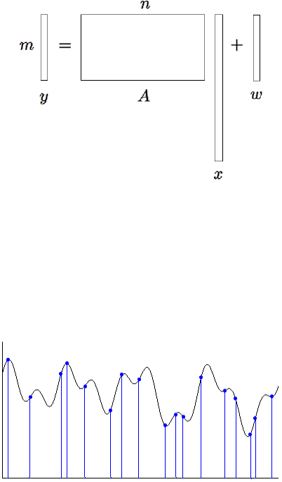
10.1 High-dimensional signal recovery problems 251
measurement matrix A in (10.1) is a realization of a random matrix drawn from
some distribution. More specifically, we assume that the rows A
i
are independent
random vectors, which makes the observations y
i
independent, too.
Figure 10.1 Signal recovery problem: recover a signal x from random,
linear measurements y.
Example 10.1.1 (Audio sampling). In signal processing applications, x can be
a digitized audio signal. The measurement vector y can be obtained by sampling
x at m randomly chosen time points, see Figure 10.2.
Figure 10.2 Signal recovery problem in audio sampling: recover an audio
signal x from a sample of x taken at m random time points.
Example 10.1.2 (Linear regression). The linear regression is one of the major
inference problems in Statistics. Here we would like to model the relationship
between n predictor variables and a response variable using a sample of m obser-
vations. The regression problem is usually written as
Y = Xβ + w.
Here X is an m ×n matrix that contains a sample of predictor variables, Y ∈ R
m
is a vector that contains a sample of response variables, β ∈ R
n
is a coefficient
vector that specifies the relationship that we try to recover, and w is a noise
vector.
252 Sparse Recovery
For example, in genetics one could be interested in predicting a certain disease
based on genetic information. One then performs a study on m patients collecting
the expressions of their n genes. The matrix X is defined by letting X
ij
be the
expression of gene j in patient i, and the coefficients Y
i
of the vector Y can be set
to quantify whether or not patient i has the disease (and to what extent). The
goal is to recover the coefficients of β, which quantify how each gene affects the
disease.
10.1.1 Incorporating prior information about the signal
Many modern signal recovery problems operate in the regime where
m ≪ n,
i.e. we have far fewer measurements than unknowns. For instance, in a typical
genetic study like the one described in Example 10.1.2, the number of patients is
∼ 100 while the number of genes is ∼ 10, 000.
In this regime, the recovery problem (10.1) is ill-posed even in the noiseless
case where w = 0. It can not be even approximately solved: the solutions form a
linear subspace of dimension at least n − m. To overcome this difficulty, we can
leverage some prior information about the signal x – something that we know,
believe, or want to enforce about x. Such information can be mathematically be
expressed by assuming that
x ∈ T (10.3)
where T ⊂ R
n
is a known set.
The smaller the set T, the fewer measurements m could be needed to recover x.
For small T , we can hope that signal recovery can be solved even in the ill-posed
regime where m ≪ n. We see how this idea works in the next sections.
10.2 Signal recovery based on M
∗
bound
Let us return to the the recovery problem (10.1). For simplicity, let us first con-
sider the noiseless version of the problem, that is
y = Ax, x ∈ T.
To recap, here x ∈ R
n
is the unknown signal, T ⊂ R
n
is a known set that encodes
our prior information about x, and A is a known m × n random measurement
matrix. Our goal is to recover x from y.
Perhaps the simplest candidate for the solution would be any vector x
′
that is
consistent both with the measurements and the prior, so we
find x
′
:
y = Ax
′
, x
′
∈ T. (10.4)
If the set T is convex, this is a convex program (in the feasibility form), and many
effective algorithms exists to numerically solve it.

10.2 Signal recovery based on M
∗
bound 253
This na¨ıve approach actually works well. We now quickly deduce this from the
M
∗
bound from Section 9.4.1.
Theorem 10.2.1. Suppose the rows A
i
of A are independent, isotropic and sub-
gaussian random vectors. Then any solution
b
x of the program (10.4) satisfies
E ∥
b
x − x∥
2
≤
CK
2
w(T)
√
m
,
where K = max
i
∥A
i
∥
ψ
2
.
Proof Since x,
b
x ∈ T and Ax = A
b
x = y, we have
x,
b
x ∈ T ∩ E
x
where E
x
:
= x + ker A. (Figure 10.3 illustrates this situation visually.) Then the
Figure 10.3 Signal recovery: the signal x and the solution bx lie in the prior
set T and in the affine subspace E
x
.
affine version of the M
∗
bound (Exercise 9.4.3) yields
E ∥
b
x − x∥
2
≤ E diam(T ∩ E
x
) ≤
CK
2
w(T)
√
m
.
This completes the proof.
Remark 10.2.2 (Stable dimension). Arguing as in Remark 9.4.4, we obtain a
non-trivial error bound
E ∥
b
x − x∥
2
≤ ε · diam(T )
provided that the number of measurements m is so that
m ≥ C(K
4
/ε
2
)d(T ).
In words, the signal can be approximately recovered as long as the number of
measurements m exceeds a multiple of the stable dimension d(T ) of the prior set
T .
Since the stable dimension can be much smaller than the ambient dimension n,
the recovery problem may often be solved even in the high-dimensional, ill-posed
regime where
m ≪ n.
We see some concrete examples of this situation shortly.

254 Sparse Recovery
Remark 10.2.3 (Convexity). If the prior set T is not convex, we can convexify it
by replacing T with its convex hull conv(T ). This makes (10.4) a convex program,
and thus computationally tractable. At the same time, the recovery guarantees
of Theorem 10.2.1 do not change since
w(conv(T )) = w(T )
by Proposition 7.5.2.
Exercise 10.2.4 (Noisy measurements). KK Extend the recovery result (The-
orem 10.2.1) for the noisy model y = Ax + w we considered in (10.1). Namely,
show that
E ∥
b
x − x∥
2
≤
CK
2
w(T) + ∥w∥
2
√
m
.
Hint: Modify the argument that leads to the M
∗
bound.
Exercise 10.2.5 (Mean squared error). KKK Prove that the error bound The-
orem 10.2.1 can be extended for the mean squared error
E ∥
b
x − x∥
2
2
.
Hint: Modify the M
∗
bound accordingly.
Exercise 10.2.6 (Recovery by optimization). Suppose T is the unit ball of some
norm ∥·∥
T
in R
n
. Show that the conclusion of Theorem 10.2.1 holds also for the
solution of the following optimization program:
minimize ∥x
′
∥
T
s.t. y = Ax
′
.
10.3 Recovery of sparse signals
10.3.1 Sparsity
Let us give a concrete example of a prior set T . Very often, we believe that x
should be sparse, i.e. that most coefficients of x are zero, exactly or approximately.
For instance, in genetic studies like the one we described in Example 10.1.2, it is
natural to expect that very few genes (∼ 10) have significant impact on a given
disease, and we would like to find out which ones.
In some applications, one needs to change the basis so that the signals of
interest are sparse. For instance, in the audio recovery problem considered in
Example 10.1.1, we typically deal with band-limited signals x. Those are the
signals whose frequencies (the values of the Fourier transform) are constrained
to some small set, such as a bounded interval. While the audio signal x itself is
not sparse as is apparent from Figure 10.2, the Fourier transform of x may be
sparse. In other words, x may be sparse in the frequency and not time domain.
To quantify the (exact) sparsity of a vector x ∈ R
n
, we consider the size of the
support of x which we denote
∥x∥
0
:
= |supp(x)| =
{i
:
x
i
̸= 0}
.
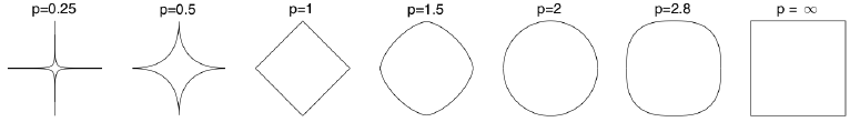
10.3 Recovery of sparse signals 255
Assume that
∥x∥
0
= s ≪ n. (10.5)
This can be viewed as a special case of a general assumption (10.3) by putting
T =
x ∈ R
n
:
∥x∥
0
≤ s
.
Then a simple dimension count shows the recovery problem (10.1) could become
well posed:
Exercise 10.3.1 (Sparse recovery problem is well posed). KKK Argue that
if A is in general position and m ≥ 2∥x∥
0
, the solution to the sparse recovery
problem (10.1) is unique if it exists. (Choose a useful definition of general position
for this problem.)
Even when the problem (10.1) is well posed, it could be computationally hard.
It is easy if one knows the support of x (why?) but usually the support is unknown.
An exhaustive search over all possible supports (subsets of a given size s) is
impossible since the number of possibilities is exponentially large:
n
s
≥ 2
s
.
Fortunately, there exist computationally effective approaches to high-dimensional
recovery problems with general constraints (10.3), and the sparse recovery prob-
lems in particular. We cover these approaches next.
Exercise 10.3.2 (The “ℓ
p
norms” for 0 ≤ p < 1). KKK
(a) Check that ∥ · ∥
0
is not a norm on R
n
.
(b) Check that ∥ · ∥
p
is not a norm on R
n
if 0 < p < 1. Figure 10.4 illustrates
the unit balls for various ℓ
p
“norms”.
(c) Show that, for every x ∈ R
n
,
∥x∥
0
= lim
p→0
+
∥x∥
p
p
.
Figure 10.4 The unit balls of ℓ
p
for various p in R
2
.
10.3.2 Convexifying the sparsity by ℓ
1
norm, and recovery guarantees
Let us specialize the general recovery guarantees developed in Section 10.2 to the
sparse recovery problem. To do this, we should choose the prior set T so that it
promotes sparsity. In the previous section, we saw that the choice
T
:
=
x ∈ R
n
:
∥x∥
0
≤ s

256 Sparse Recovery
does not allow for computationally tractable algorithms.
To make T convex, we may replace the “ℓ
0
norm” by the ℓ
p
norm with the
smallest exponent p > 0 that makes this a true norm. This exponent is obviously
p = 1 as we can see from Figure 10.4. So let us repeat this important heuristic:
we propose to replace the ℓ
0
“norm” by the ℓ
1
norm.
Thus it makes sense to choose T to be a scaled ℓ
1
ball:
T
:
=
√
sB
n
1
.
The scaling factor
√
s was chosen so that T can accommodate all s-sparse unit
vectors:
Exercise 10.3.3. K Check that
x ∈ R
n
:
∥x∥
0
≤ s, ∥x∥
2
≤ 1
⊂
√
sB
n
1
.
For this T , the general recovery program (10.4) becomes
Find x
′
:
y = Ax
′
, ∥x
′
∥
1
≤
√
s. (10.6)
Note that this is a convex program, and therefore is computationally tractable.
And the general recovery guarantee, Theorem 10.2.1, specialized to our case,
implies the following.
Corollary 10.3.4 (Sparse recovery: guarantees). Assume the unknown s-sparse
signal x ∈ R
n
satisfies ∥x∥
2
≤ 1. Then x can be approximately recovered from the
random measurement vector y = Ax by a solution
b
x of the program (10.6). The
recovery error satisfies
E ∥
b
x − x∥
2
≤ CK
2
r
s log n
m
.
Proof Set T =
√
sB
n
1
. The result follows from Theorem 10.2.1 and the bound
(7.18) on the Gaussian width of the ℓ
1
ball:
w(T) =
√
sw(B
n
1
) ≤ C
p
s log n.
Remark 10.3.5. The recovery error guaranteed by Corollary 10.3.4 is small if
m ≳ s log n
(if the hidden constant here is appropriately large). In words, recovery is possible
if the number of measurements m is almost linear in the sparsity s, while its
dependence on the ambient dimension n is mild (logarithmic). This is good news.
It means that for sparse signals, one can solve recovery problems in the high-
dimensional regime where
m ≪ n,
i.e. with much fewer measurements than the dimension.
Exercise 10.3.6 (Sparse recovery by convex optimization). KKK

10.3 Recovery of sparse signals 257
(a) Show that an unknown s-sparse signal x (without restriction on the norm)
can be approximately recovered by solving the convex optimization prob-
lem
minimize ∥x
′
∥
1
s.t. y = Ax
′
. (10.7)
The recovery error satisfies
E ∥
b
x − x∥
2
≤ CK
2
r
s log n
m
∥x∥
2
.
(b) Argue that a similar result holds for approximately sparse signals. State
and prove such a guarantee.
10.3.3 The convex hull of sparse vectors, and the logarithmic
improvement
The replacement of s-sparse vectors by the octahedron
√
sB
n
1
that we made in
Exercise 10.3.3 is almost sharp. In the following exercise, we show that the convex
hull of the set of sparse vectors
S
n,s
:
=
x ∈ R
n
:
∥x∥
0
≤ s, ∥x∥
2
≤ 1
is approximately the truncated ℓ
1
ball
T
n,s
:
=
√
sB
n
1
∩ B
n
2
=
n
x ∈ R
n
:
∥x∥
1
≤
√
s, ∥x∥
2
≤ 1
o
.
Exercise 10.3.7 (The convex hull of sparse vectors). KKK
(a) Check that
conv(S
n,s
) ⊂ T
n,s
.
(b) To help us prove a reverse inclusion, fix x ∈ T
n,s
and partition the support
of x into disjoint subsets I
1
, I
2
, . . . so that I
1
indexes the s largest coeffi-
cients of x in magnitude, I
2
indexes the next s largest coefficients, and so
on. Show that
X
i≥1
∥x
I
i
∥
2
≤ 2,
where x
I
∈ R
T
denotes the restriction of x onto a set I.
Hint: Note that ∥x
I
1
∥
2
≤ 1. Next, for i ≥ 2, note that each coordinate of x
I
i
is smaller in
magnitude than the average coordinate of x
I
i−1
; conclude that ∥x
I
i
∥
2
≤ (1/
√
s)∥x
I
i−1
∥
1
. Then
sum up the bounds.
(c) Deduce from part 2 that
T
n,s
⊂ 2 conv(S
n,s
).
Exercise 10.3.8 (Gaussian width of the set of sparse vectors). KK Use Exer-
cise 10.3.7 to show that
w(T
n,s
) ≤ 2w(S
n,s
) ≤ C
q
s log(en/s).

258 Sparse Recovery
Improve the logarithmic factor in the error bound for sparse recovery (Corol-
lary 10.3.4) to
E ∥
b
x − x∥
2
≤ C
r
s log(en/s)
m
.
This shows that
m ≳ s log(en/s)
measurements suffice for sparse recovery.
Exercise 10.3.9 (Sharpness). KKKK Show that
w(T
n,s
) ≥ w(S
n,s
) ≥ c
q
s log(2n/s).
Hint: Construct a large ε-separated subset of S
n,s
and thus deduce a lower bound on the covering
numbers of S
n,s
. Then use Sudakov’s minoration inequality (Theorem 7.4.1 .
Exercise 10.3.10 (Garnaev-Gluskin’s theorem). KKK Improve the logarith-
mic factor in the bound (9.4.5) on the sections of the ℓ
1
ball. Namely, show that
E diam(B
n
1
∩ E) ≲
r
log(en/m)
m
.
In particular, this shows that the logarithmic factor in (9.16) is not needed.
Hint: Fix ρ > 0 and apply the M
∗
bound for the truncated octahedron T
ρ
:
= B
n
1
∩ ρB
n
2
. Use Exer-
cise 10.3.8 to bound the Gaussian width of T
ρ
. Furthermore, note that if rad(T
ρ
∩E) ≤ δ for some δ ≤ ρ
then rad(T ∩ E) ≤ δ. Finally, optimize in ρ.
10.4 Low-rank matrix recovery
In the following series of exercises, we establish a matrix version of the sparse
recovery problem studied in Section 10.3. The unknown signal will now be a d×d
matrix X instead of a signal x ∈ R
n
considered previously.
There are two natural notions of sparsity for matrices. One is where most of
the entries of X are zero, and this can be quantified by the ℓ
0
“norm” ∥X∥
0
,
which counts non-zero entries. For this notion, we can directly apply the analysis
of sparse recovery from Section 10.3. Indeed, it is enough to vectorize the matrix
X and think of it as a long vector in R
d
2
.
But in this section, we consider an alternative and equally useful notion of
sparsity for matrices: low rank. It is quantified by the rank of X, which we may
think of as the ℓ
0
norm of the vector of the singular values of X, i.e.
s(X)
:
= (s
i
(X))
d
i=1
. (10.8)
Our analysis of the low-rank matrix recovery problem will roughly go along the
same lines as the analysis of sparse recovery, but will not be identical to it.
Let us set up a low-rank matrix recovery problem. We would like to recover an
unknown d × d matrix from m random measurements of the form
y
i
= ⟨A
i
, X⟩, i = 1, . . . , m. (10.9)

10.4 Low-rank matrix recovery 259
Here A
i
are independent d ×d matrices, and ⟨A
i
, X⟩ = tr(A
T
i
X) is the canonical
inner product of matrices (recall Section 4.1.3). In dimension d = 1, the matrix
recovery problem (10.9) reduces to the vector recovery problem (10.2).
Since we have m linear equations in d×d variables, the matrix recovery problem
is ill-posed if
m < d
2
.
To be able to solve it in this range, we make an additional assumption that X
has low rank, i.e.
rank(X) ≤ r ≪ d.
10.4.1 The nuclear norm
Like sparsity, the rank is not a convex function. To fix this, in Section 10.3 we
replaced the sparsity (i.e. the ℓ
0
“norm”) by the ℓ
1
norm. Let us try to do the
same for the notion of rank. The rank of X is the ℓ
0
“norm” of the vector s(X)
of the singular values in (10.8). Replacing the ℓ
0
norm by the ℓ
1
norm, we obtain
the quantity
∥X∥
∗
:
= ∥s(X)∥
1
=
d
X
i=1
s
i
(X) = tr
√
X
T
X
which is called the nuclear norm, or trace norm, of X. (We omit the absolute
values since the singular values are non-negative.)
Exercise 10.4.1. KKK Prove that ∥·∥
∗
is indeed a norm on the space of d×d
matrices.
Hint: This will follow once you check the identity ∥X∥
∗
= max
|⟨X, U⟩|
:
U ∈ O(d)
where O(d)
denotes the set of d × d orthogonal matrices. Prove the identity using the singular value decomposition
of X.
Exercise 10.4.2 (Nuclear, Frobenius and operator norms). KK Check that
⟨X, Y ⟩ ≤ ∥X∥
∗
· ∥Y ∥ (10.10)
Conclude that
∥X∥
2
F
≤ ∥X∥
∗
· ∥X∥.
Hint: Think of the nuclear norm ∥ · ∥
∗
, Frobenius norm ∥ · ∥
F
and the operator norm ∥ · ∥ as matrix
analogs of the ℓ
1
norm, ℓ
2
norm and ℓ
∞
norms for vectors, respectively.
Denote the unit ball of the nuclear norm by
B
∗
:
=
n
X ∈ R
d×d
:
∥X∥
∗
≤ 1
o
.
Exercise 10.4.3 (Gaussian width of the unit ball of the nuclear norm). K Show
that
w(B
∗
) ≤ 2
√
d.
Hint: Use (10.10) followed by Theorem 7.3.1.

260 Sparse Recovery
The following is a matrix version of Exercise 10.3.3.
Exercise 10.4.4. K Check that
n
X ∈ R
d×d
:
rank(X) ≤ r, ∥X∥
F
≤ 1
o
⊂
√
rB
∗
.
10.4.2 Guarantees for low-rank matrix recovery
It makes sense to try to solve the low-rank matrix recovery problem (10.9) using
the matrix version of the convex program (10.6), i.e.
Find X
′
:
y
i
=
A
i
, X
′
∀i = 1, . . . , m; ∥X
′
∥
∗
≤
√
r. (10.11)
Exercise 10.4.5 (Low-rank matrix recovery: guarantees). KK Suppose the
random matrices A
i
are independent and have all independent, sub-gaussian en-
tries.
1
Assume the unknown d×d matrix X with rank r satisfies ∥X∥
F
≤ 1. Show
that X can be approximately recovered from the random measurements y
i
by a
solution
b
X of the program (10.11). Show that the recovery error satisfies
E ∥
b
X − X∥
F
≤ CK
2
r
rd
m
.
Remark 10.4.6. The recovery error becomes small if
m ≳ rd,
if the hidden constant here is appropriately large. This allows us to recover low-
rank matrices even when the number of measurements m is too small, i.e. when
m ≪ d
2
and the matrix recovery problem (without rank assumption) is ill-posed.
Exercise 10.4.7. KK Extend the matrix recovery result for approximately low-
rank matrices.
The following is a matrix version of Exercise 10.3.6.
Exercise 10.4.8 (Low-rank matrix recovery by convex optimization). KK Show
that an unknown matrix X of rank r can be approximately recovered by solving
the convex optimization problem
minimize ∥X
′
∥
∗
s.t. y
i
=
A
i
, X
′
∀i = 1, . . . , m.
Exercise 10.4.9 (Rectangular matrices). KK Extend the matrix recovery re-
sult from quadratic to rectangular, d
1
× d
2
matrices.
1
The independence of entries can be relaxed. How?

10.5 Exact recovery and the restricted isometry property 261
10.5 Exact recovery and the restricted isometry property
It turns out that the guarantees for sparse recovery we just developed can be
dramatically improved: the recovery error for sparse signals x can actually be zero!
We discuss two approaches to this remarkable phenomenon. First we deduce exact
recovery from Escape Theorem 9.4.7. Next we present a general deterministic
condition on a matrix A which guarantees exact recovery; it is known as the
restricted isometry property (RIP). We check that random matrices A satisfy
RIP, which gives another approach to exact recovery.
10.5.1 Exact recovery based on the Escape Theorem
To see why exact recovery should be possible, let us look at the recovery problem
from a geometric viewpoint illustrated by Figure 10.3. A solution
b
x of the program
(10.6) must lie in the intersection of the prior set T , which in our case is the ℓ
1
ball
√
sB
n
1
, and the affine subspace E
x
= x + ker A.
The ℓ
1
ball is a polytope, and the s-sparse unit vector x lies on the s − 1-
dimensional edge of that polytope, see Figure 10.5a.
(a) Exact sparse recovery happens when
the random subspace E
x
is tangent to the
ℓ
1
ball at the point x.
(b) The tangency occurs iff E
x
is disjoint
from the spherical part S(x) of the tan-
gent cone T (x) of the ℓ
1
ball at point x.
Figure 10.5 Exact sparse recovery
It could happen with non-zero probability that the random subspace E
x
is
tangent to the polytope at the point x. If this does happen, x is the only point of
intersection between the ℓ
1
ball and E
x
. In this case, it follows that the solution
b
x to the program (10.6) is exact:
b
x = x.
To justify this argument, all we need to check is that a random subspace E
x
is tangent to the ℓ
1
ball with high probability. We can do this using Escape
Theorem 9.4.7. To see a connection, look at what happens in a small neighborhood
around the tangent point, see Figure 10.5b. The subspace E
x
is tangent if and
only if the tangent cone T (x) (formed by all rays emanating from x toward the
points in the ℓ
1
ball) intersects E
x
at a single point x. Equivalently, this happens
if and only if the spherical part S(x) of the cone (the intersection of T (x) with a

262 Sparse Recovery
small sphere centered at x) is disjoint from E
x
. But this is exactly the conclusion
of Escape Theorem 9.4.7!
Let us now formally state the exact recovery result. We shall consider the
noiseless sparse recovery problem
y = Ax.
and try to solve it using the optimization program (10.7), i.e.
minimize ∥x
′
∥
1
s.t. y = Ax
′
. (10.12)
Theorem 10.5.1 (Exact sparse recovery). Suppose the rows A
i
of A are inde-
pendent, isotropic and sub-gaussian random vectors, and let K
:
= max
i
∥A
i
∥
ψ
2
.
Then the following happens with probability at least 1 − 2 exp(−cm/K
4
).
Assume an unknown signal x ∈ R
n
is s-sparse and the number of measurements
m satisfies
m ≥ CK
4
s log n.
Then a solution
b
x of the program (10.12) is exact, i.e.
b
x = x.
To prove the theorem, we would like to show that the recovery error
h
:
=
b
x − x
is zero. Let us examine the vector h more closely. First we show that h has more
“energy” on the support of x than outside it.
Lemma 10.5.2. Let S
:
= supp(x). Then
∥h
S
c
∥
1
≤ ∥h
S
∥
1
.
Here h
S
∈ R
S
denotes the restriction of the vector h ∈ R
n
onto a subset of
coordinates S ⊂ {1, . . . , n}.
Proof Since
b
x is the minimizer in the program (10.12), we have
∥
b
x∥
1
≤ ∥x∥
1
. (10.13)
But there is also a lower bound
∥
b
x∥
1
= ∥x + h∥
1
= ∥x
S
+ h
S
∥
1
+ ∥x
S
c
+ h
S
c
∥
1
≥ ∥x∥
1
− ∥h
S
∥
1
+ ∥h
S
c
∥
1
,
where the last line follows by triangle inequality and using x
S
= x and x
S
c
= 0.
Substitute this bound into (10.13) and cancel ∥x∥
1
on both sides to complete the
proof.
Lemma 10.5.3. The error vector satisfies
∥h∥
1
≤ 2
√
s∥h∥
2
.

10.5 Exact recovery and the restricted isometry property 263
Proof Using Lemma 10.5.2 and then Cauchy-Schwarz inequality, we obtain
∥h∥
1
= ∥h
S
∥
1
+ ∥h
S
c
∥
1
≤ 2∥h
S
∥
1
≤ 2
√
s∥h
S
∥
2
.
Since trivially ∥h
S
∥
2
≤ ∥h∥
2
, the proof is complete.
Proof of Theorem 10.5.1 Assume that the recovery is not exact, i.e.
h =
b
x − x ̸= 0.
By Lemma 10.5.3, the normalized error h/∥h∥
2
lies in the set
T
s
:
=
n
z ∈ S
n−1
:
∥z∥
1
≤ 2
√
s
o
.
Since also
Ah = A
b
x − Ax = y − y = 0,
we have
h
∥h∥
2
∈ T
s
∩ ker A. (10.14)
Escape Theorem 9.4.7 states that this intersection is empty with high proba-
bility, as long as
m ≥ CK
4
w(T
s
)
2
.
Now,
w(T
s
) ≤ 2
√
sw(B
n
1
) ≤ C
p
s log n, (10.15)
where we used the bound (7.18) on the Gaussian width of the ℓ
1
ball. Thus,
if m ≥ CK
4
s log n, the intersection in (10.14) is empty with high probability,
which means that the inclusion in (10.14) can not hold. This contradiction implies
that our assumption that h ̸= 0 is false with high probability. The proof is
complete.
Exercise 10.5.4 (Improving the logarithmic factor). K Show that the con-
clusion of Theorem 10.5.1 holds under a weaker assumption on the number of
measurements, which is
m ≥ CK
4
s log(en/s).
Hint: Use the result of Exercise 10.3.8.
Exercise 10.5.5. KK Give a geometric interpretation of the proof of Theo-
rem 10.5.1, using Figure 10.5b. What does the proof say about the tangent cone
T (x)? Its spherical part S(x)?
Exercise 10.5.6 (Noisy measurements). KKK Extend the result on sparse
recovery (Theorem 10.5.1) for noisy measurements, where
y = Ax + w.
You may need to modify the recovery program by making the constraint y = Ax
′
approximate?
264 Sparse Recovery
Remark 10.5.7. Theorem 10.5.1 shows that one can effectively solve under-
determined systems of linear equations y = Ax with m ≪ n equations in n
variables, if the solution is sparse.
10.5.2 Restricted isometries
This subsection is optional; the further material is not based on it.
All recovery results we proved so far were probabilistic: they were valid for
a random measurement matrix A and with high probability. We may wonder if
there exists a deterministic condition which can guarantee that a given matrix A
can be used for sparse recovery. Such condition is the restricted isometry property
(RIP).
Definition 10.5.8 (RIP). An m × n matrix A satisfies the restricted isometry
property (RIP) with parameters α, β and s if the inequality
α∥v∥
2
≤ ∥Av∥
2
≤ β∥v∥
2
holds for all vectors v ∈ R
n
such that
2
∥v∥
0
≤ s.
In other words, a matrix A satisfies RIP if the restriction of A on any s-
dimensional coordinate subspace of R
n
is an approximate isometry in the sense
of (4.5).
Exercise 10.5.9 (RIP via singular values). K Check that RIP holds if and
only if the singular values satisfy the inequality
α ≤ s
s
(A
I
) ≤ s
1
(A
I
) ≤ β
for all subsets I ⊂ [n] of size |I| = s. Here A
I
denotes the m ×s sub-matrix of A
formed by selecting the columns indexed by I.
Now we prove that RIP is indeed a sufficient condition for sparse recovery.
Theorem 10.5.10 (RIP implies exact recovery). Suppose an m × n matrix A
satisfies RIP with some parameters α, β and (1 + λ)s, where λ > (β/α)
2
. Then
every s-sparse vector x ∈ R
n
can be recovered exactly by solving the program
(10.12), i.e. the solution satisfies
b
x = x.
Proof As in the proof of Theorem 10.5.1, we would like to show that the recovery
error
h =
b
x − x
is zero. To do this, we decompose h in a way similar to Exercise 10.3.7.
Step 1: decomposing the support. Let I
0
be the support of x; let I
1
index
the λs largest coefficients of h
I
c
0
in magnitude; let I
2
index the next λs largest
coefficients of h
I
c
0
in magnitude, and so on. Finally, denote I
0,1
= I
0
∪ I
1
.
2
Recall from Section 10.3.1 that by ∥v∥
0
we denote the number of non-zero coordinates of v.

10.5 Exact recovery and the restricted isometry property 265
Since
Ah = A
b
x − Ax = y − y = 0,
triangle inequality yields
0 = ∥Ah∥
2
≥ ∥A
I
0,1
h
I
0,1
∥
2
− ∥A
I
c
0,1
h
I
c
0,1
∥
2
. (10.16)
Next, we examine the two terms in the right side.
Step 2: applying RIP. Since |I
0,1
| ≤ s + λs, RIP yields
∥A
I
0,1
h
I
0,1
∥
2
≥ α∥h
I
0,1
∥
2
and triangle inequality followed by RIP also give
∥A
I
c
0,1
h
I
c
0,1
∥
2
≤
X
i≥2
∥A
I
i
h
I
i
∥
2
≤ β
X
i≥2
∥h
I
i
∥
2
.
Plugging into (10.16) gives
β
X
i≥2
∥h
I
i
∥
2
≥ α∥h
I
0,1
∥
2
. (10.17)
Step 3: summing up. Next, we bound the sum in the left like we did in
Exercise 10.3.7. By definition of I
i
, each coefficient of h
I
i
is bounded in magnitude
by the average of the coefficients of h
I
i−1
, i.e. by ∥h
I
i−1
∥
1
/(λs) for i ≥ 2. Thus
∥h
I
i
∥
2
≤
1
√
λs
∥h
I
i−1
∥
1
.
Summing up, we get
X
i≥2
∥h
I
i
∥
2
≤
1
√
λs
X
i≥1
∥h
I
i
∥
1
=
1
√
λs
∥h
I
c
0
∥
1
≤
1
√
λs
∥h
I
0
∥
1
(by Lemma 10.5.2)
≤
1
√
λ
∥h
I
0
∥
2
≤
1
√
λ
∥h
I
0,1
∥
2
.
Putting this into (10.17) we conclude that
β
√
λ
∥h
I
0,1
∥
2
≥ α∥h
I
0,1
∥
2
.
This implies that h
I
0,1
= 0 since β/
√
λ < α by assumption. By construction, I
0,1
contains the largest coefficient of h. It follows that h = 0 as claimed. The proof
is complete.
Unfortunately, it is unknown how to construct deterministic matrices A that
satisfy RIP with good parameters (i.e. with β = O(α) and with s as large as m,
up to logarithmic factors). However, it is quite easy to show that random matrices
A do satisfy RIP with high probability:

266 Sparse Recovery
Theorem 10.5.11 (Random matrices satisfy RIP). Consider an m×n matrix A
whose rows A
i
of A are independent, isotropic and sub-gaussian random vectors,
and let K
:
= max
i
∥A
i
∥
ψ
2
. Assume that
m ≥ CK
4
s log(en/s).
Then, with probability at least 1 −2 exp(−cm/K
4
), the random matrix A satisfies
RIP with parameters α = 0.9
√
m, β = 1.1
√
m and s.
Proof By Exercise 10.5.9, it is enough to control the singular values of all m ×s
sub-matrices A
I
. We will do it by using the two-sided bound from Theorem 4.6.1
and then taking the union bound over all sub-matrices.
Let us fix I. Theorem 4.6.1 yields
√
m − r ≤ s
s
(A
I
) ≤ s
1
(A
I
) ≤
√
m + r
with probability at least 1 − 2 exp(−t
2
), where r = C
0
K
2
(
√
s + t). If we set t =
√
m/(20C
0
K
2
) and use the assumption on m with appropriately large constant
C, we can make sure that r ≤ 0.1
√
m. This yields
0.9
√
m ≤ s
s
(A
I
) ≤ s
1
(A
I
) ≤ 1.1
√
m (10.18)
with probability at least 1 − 2 exp(−2cm
2
/K
4
), where c > 0 is an absolute con-
stant.
It remains to take a union bound over all s-element subsets I ⊂ [n]; there are
n
s
of them. We conclude that (10.18) holds with probability at least
1 − 2 exp(−2cm
2
/K
4
) ·
n
s
!
> 1 − 2 exp(−cm
2
/K
4
).
To get the last inequality, recall that
n
s
≤ exp(s log(en/s)) by (0.0.5) and use
the assumption on m. The proof is complete.
The results we just proved give another approach to Theorem 10.5.1 about
exact recovery with a random matrix A.
Second proof of Theorem 10.5.1 By Theorem 10.5.11, A satisfies RIP with α =
0.9
√
m, β = 1.1
√
m and 3s. Thus, Theorem 10.5.10 for λ = 2 guarantees exact
recovery. We conclude that Theorem 10.5.1 holds, and we even get the logarithmic
improvement noted in Exercise 10.5.4.
An advantage of RIP is that this property is often simpler to verify than to
prove exact recovery directly. Let us give one example.
Exercise 10.5.12 (RIP for random projections). KKK Let P be the orthog-
onal projection in R
n
onto an m-dimensional random subspace uniformly dis-
tributed in the Grassmanian G
n,m
.
(a) Prove that P satisfies RIP with good parameters (similar to Theorem 10.5.11,
up to a normalization).
(b) Conclude a version of Theorem 10.5.1 for exact recovery from random
projections.
10.6 Lasso algorithm for sparse regression 267
10.6 Lasso algorithm for sparse regression
In this section we analyze an alternative method for sparse recovery. This method
was originally developed in statistics for the equivalent problem of sparse linear
regression, and it is called Lasso (“least absolute shrinkage and selection opera-
tor”).
10.6.1 Statistical formulation
Let us recall the classical linear regression problem, which we described in Ex-
ample 10.1.2. It is
Y = Xβ + w (10.19)
where X is a known m × n matrix that contains a sample of predictor variables,
Y ∈ R
m
is a known vector that contains a sample of the values of the response
variable, β ∈ R
n
is an unknown coefficient vector that specifies the relationship
between predictor and response variables, and w is a noise vector. We would like
to recover β.
If we do not assume anything else, the regression problem can be solved by the
method of ordinary least squares, which minimizes the ℓ
2
-norm of the error over
all candidates for β:
minimize ∥Y − Xβ
′
∥
2
s.t. β
′
∈ R
n
. (10.20)
Now let us make an extra assumption that β
′
is sparse, so that the response
variable depends only on a few of the n predictor variables (e.g. the cancer de-
pends on few genes). So, like in (10.5), we assume that
∥β∥
0
≤ s
for some s ≪ n. As we argued in Section 10.3, the ℓ
0
is not convex, and its convex
proxy is the ℓ
1
norm. This prompts us to modify the ordinary least squares pro-
gram (10.20) by including a restriction on the ℓ
1
norm, which promotes sparsity
in the solution:
minimize ∥Y − Xβ
′
∥
2
s.t. ∥β
′
∥
1
≤ R, (10.21)
where R is a parameter which specifies a desired sparsity level of the solution. The
program (10.21) is one of the formulations of Lasso, the most popular statistical
method for sparse linear regression. It is a convex program, and therefore is
computationally tractable.
10.6.2 Mathematical formulation and guarantees
It would be convenient to return to the notation we used for sparse recovery
instead of using the statistical notation in the previous section. So let us restate
the linear regression problem (10.19) as
y = Ax + w

268 Sparse Recovery
where A is a known m×n matrix, y ∈ R
m
is a known vector, x ∈ R
n
is an unknown
vector that we are trying to recover, and w ∈ R
m
is noise which is either fixed or
random and independent of A. Then Lasso program (10.21) becomes
minimize ∥y − Ax
′
∥
2
s.t. ∥x
′
∥
1
≤ R. (10.22)
We prove the following guarantee of the performance of Lasso.
Theorem 10.6.1 (Performance of Lasso). Suppose the rows A
i
of A are inde-
pendent, isotropic and sub-gaussian random vectors, and let K
:
= max
i
∥A
i
∥
ψ
2
.
Then the following happens with probability at least 1 − 2 exp(−s log n).
Assume an unknown signal x ∈ R
n
is s-sparse and the number of measurements
m satisfies
m ≥ CK
4
s log n. (10.23)
Then a solution
b
x of the program (10.22) with R
:
= ∥x∥
1
is accurate, namely
∥
b
x − x∥
2
≤ Cσ
r
s log n
m
,
where σ = ∥w∥
2
/
√
m.
Remark 10.6.2 (Noise). The quantity σ
2
is the average squared noise per mea-
surement, since
σ
2
=
∥w∥
2
2
m
=
1
m
m
X
i=1
w
2
i
.
Then, if the number of measurements is
m ≳ s log n,
Theorem 10.6.1 bounds the recovery error by the average noise per measurement
σ. And if m is larger, the recovery error gets smaller.
Remark 10.6.3 (Exact recovery). In the noiseless model y = Ax we have w = 0
and thus Lasso recovers x exactly, i.e.
b
x = x.
The proof of Theorem 10.6.1 will be similar to our proof of Theorem 10.5.1 on
exact recovery, although instead of the Escape theorem we use Matrix Deviation
Inequality (Theorem 9.1.1) directly this time.
We would like to bound the norm of the error vector
h
:
=
b
x − x.
Exercise 10.6.4. KK Check that h satisfies the conclusions of Lemmas 10.5.2
and 10.5.3, so we have
∥h∥
1
≤ 2
√
s∥h∥
2
. (10.24)
Hint: The proofs of these lemmas are based on the fact that ∥bx∥
1
≤ ∥x∥
1
, which holds in our situation
as well.

10.6 Lasso algorithm for sparse regression 269
In case where the noise w is nonzero, we can not expect to have Ah = 0 like in
Theorem 10.5.1. (Why?) Instead, we can give an upper and a lower bounds for
∥Ah∥
2
.
Lemma 10.6.5 (Upper bound on ∥Ah∥
2
). We have
∥Ah∥
2
2
≤ 2
D
h, A
T
w
E
. (10.25)
Proof Since
b
x is the minimizer of Lasso program (10.22), we have
∥y − A
b
x∥
2
≤ ∥y − Ax∥
2
.
Let us express both sides of this inequality in terms of h and w, using that
y = Ax + w and h =
b
x − x:
y − A
b
x = Ax + w − A
b
x = w − Ah;
y − Ax = w.
So we have
∥w − Ah∥
2
≤ ∥w∥
2
.
Square both sides:
∥w∥
2
2
− 2 ⟨w, Ah⟩ + ∥Ah∥
2
2
≤ ∥w∥
2
2
.
Simplifying this bound completes the proof.
Lemma 10.6.6 (Lower bound on ∥Ah∥
2
). With probability at least 1−2 exp(−4s log n),
we have
∥Ah∥
2
2
≥
m
4
∥h∥
2
2
.
Proof By (10.24), the normalized error h/∥h∥
2
lies in the set
T
s
:
=
n
z ∈ S
n−1
:
∥z∥
1
≤ 2
√
s
o
.
Use matrix deviation inequality in its high-probability form (Exercise 9.1.8) with
u = 2
√
s log n. It yields that, with probability at least 1 − 2 exp(−4s log n),
sup
z∈T
s
∥Az∥
2
−
√
m
≤ C
1
K
2
w(T
s
) + 2
p
s log n
≤ C
2
K
2
p
s log n (recalling (10.15))
≤
√
m
2
(by assumption on m).
To make the last line work, choose the absolute constant C in (10.23) large
enough. By triangle inequality, this implies that
∥Az∥
2
≥
√
m
2
for all z ∈ T
s
.
Substituting z
:
= h/∥h∥
2
, we complete the proof.

270 Sparse Recovery
The last piece we need to prove Theorem 10.6.1 is an upper bound on the right
hand side of (10.25).
Lemma 10.6.7. With probability at least 1 − 2 exp(−4s log n), we have
D
h, A
T
w
E
≤ CK∥h∥
2
∥w∥
2
p
s log n. (10.26)
Proof As in the proof of Lemma 10.6.6, the normalized error satisfies
z =
h
∥h∥
2
∈ T
s
.
So, dividing both sides of (10.26) by ∥h∥
2
, we see that it is enough to bound the
supremum random process
sup
z∈T
s
D
z, A
T
w
E
with high probability. We are going to use Talagrand’s comparison inequality
(Corollary 8.6.3). This result applies for random processes with sub-gaussian
increments, so let us check this condition first.
Exercise 10.6.8. KK Show that the random process
X
t
:
=
D
t, A
T
w
E
, t ∈ R
n
,
has sub-gaussian increments, and
∥X
t
− X
s
∥
ψ
2
≤ CK∥w∥
2
· ∥t − s∥
2
.
Hint: Recall the proof of sub-gaussian Chevet’s inequality (Theorem 8.7.1).
Now we can use Talagrand’s comparison inequality in the high-probability form
(Exercise 8.6.5) for u = 2
√
s log n. We obtain that, with probability at least
1 − 2 exp(−4s log n),
sup
z∈T
s
D
z, A
T
w
E
≤ C
1
K∥w∥
2
w(T
s
) + 2
p
s log n
≤ C
2
K∥w∥
2
p
s log n (recalling (10.15)).
This completes the proof of Lemma 10.6.7.
Proof of Theorem 10.6.1. Put together the bounds in Lemmas 10.6.5, 10.6.6 and
10.26. By union bound, we have that with probability at least 1−4 exp(−4s log n),
m
4
∥h∥
2
2
≤ CK∥h∥
2
∥w∥
2
p
s log n.
Solving for ∥h∥
2
, we obtain
∥h∥
2
≤ CK
∥w∥
2
√
m
·
r
s log n
m
.
This completes the proof of Theorem 10.6.1.

10.7 Notes 271
Exercise 10.6.9 (Improving the logarithmic factor). K Show that Theorem 10.6.1
holds if log n is replaced by log(en/s), thus giving a stronger guarantee.
Hint: Use the result of Exercise 10.3.8.
Exercise 10.6.10. KK Deduce the exact recovery guarantee (Theorem 10.5.1)
directly from the Lasso guarantee (Theorem 10.6.1). The probability that you get
could be a bit weaker.
Another popular form of Lasso program (10.22) is the following unconstrained
version:
minimize ∥y − Ax
′
∥
2
2
+ λ∥x
′
∥
1
, (10.27)
This is a convex optimization problem, too. Here λ is a parameter which can
be adjusted depending on the desired level of sparsity. The method of Lagrange
multipliers shows that the constrained and unconstrained versions of Lasso are
equivalent for appropriate R and λ. This however does not immediately tell us
how to choose λ. The following exercise settles this question.
Exercise 10.6.11 (Unconstrained Lasso). KKKK Assume that the number of
measurements satisfy
m ≳ s log n.
Choose the parameter λ so that λ ≳
√
log n∥w∥
2
. Then, with high probability,
the solution
b
x of unconstrained Lasso (10.27) satisfies
∥
b
x − x∥
2
≲
λ
√
s
m
.
10.7 Notes
The applications we discussed in this chapter are drawn from two fields: sig-
nal processing (specifically, compressed sensing) and high-dimensional statistics
(more precisely, high-dimensional structured regression). The tutorial [223] offers
a unified treatment of these two kinds problems, which we followed in this chap-
ter. The survey [56] and book [78] offer a deeper introduction into compressed
sensing. The books [100, 42] discuss statistical aspects of sparse recovery.
Signal recovery based on M
∗
bound discussed in Section 10.2 is based on [223],
which has various versions of Theorem 10.2.1 and Corollary 10.3.4. Garnaev-
Gluskin’s bound from Exercise 10.3.10 was first proved in [80], see also [136] and
[78, Chapter 10].
The survey [58] offers a comprehensive overview of the low-rank matrix recovery
problem, which we discussed in Section 10.4. Our presentation is based on [223,
Section 10].
The phenomenon of exact sparse recovery we discussed in Section 10.5 goes
back to the origins of compressed sensing; see [56] and book [78] for its history
and recent developments. Our presentation of exact recovery via escape theorem
in Section 10.5.1 partly follows [223, Section 9]; see also [52, 189] and especially
272 Sparse Recovery
[208] for applications of the escape theorem to sparse recovery. One can obtain
very precise guarantees that give asymptotically sharp formulas (the so-called
phase transitions) for the number of measurements needed for signal recovery.
The first such phase transitions were identified in [68] for sparse signals and uni-
form random projection matrices A; see also [67, 64, 65, 66]. More recent work
clarified phase transitions for general feasible sets T and more general measure-
ment matrices [9, 162, 163].
The approach to exact sparse recovery based on RIP presented in Section 10.5.2
was pioneered by E. Candes and T. Tao [46]; see [78, Chapter 6] for a compre-
hensive introduction. An early form of Theorem 10.5.10 already appear in [46].
The proof we gave here was communicated to the author by Y. Plan; it is similar
to the argument of [44]. The fact that random matrices satisfy RIP (exemplified
by Theorem 10.5.11) is a backbone of compressed sensing; see [78, Section 9.1,
12.5], [222, Section 5.6].
The Lasso algorithm for sparse regression that we studies in Section 10.6 was
pioneered by R. Tibshirani [204]. The books [100, 42] offer a comprehensive in-
troduction into statistical problems with sparsity constraints; these books discuss
Lasso and its many variants. A version of Theorem 10.6.1 and some elements of its
proof can be traced to the work of P. J. Bickel, Y. Ritov and A. Tsybakov [22], al-
though their argument was not based on matrix deviation inequality. Theoretical
analysis of Lasso is also presented in [100, Chapter 11] and [42, Chapter 6].

11
Dvoretzky-Milman’s Theorem
Here we extend the matrix deviation inequality from Chapter 9 for general norms
on R
n
, and even for general sub-additive functions on R
n
. We use this result to
prove the fundamental Dvoretzky-Milman’s theorem in high-dimensional geome-
try. It helps us describe the shape of an m-dimensional random projection of an
arbitrary set T ⊂ R
n
. The answer depends on whether m is larger or smaller than
the critical dimension, which is the stable dimension d(T ). In the high-dimensional
regime (where m ≳ d(T )), the additive Johnson-Lindenstrauss that we studied
in Section 9.3.2 shows that the random projection approximately preserves the
geometry of T . In the low-dimensional regime (where m ≲ d(T ), geometry can no
longer be preserved due to “saturation”. Instead, Dvoretzky-Milman’s theorem
shows that in this regime the projected set is approximately a round ball.
11.1 Deviations of random matrices with respect to general norms
In this section we generalize the matrix deviation inequality from Section 9.1. We
replace the Euclidean norm by any positive-homogeneous, subadditive function.
Definition 11.1.1. Let V be a vector space. A function f
:
V → R is called
positive-homogeneous if
f(αx) = αf(x) for all α ≥ 0 and x ∈ V .
The function f is called subadditive if
f(x + y) ≤ f (x) + f(y) for all x, y ∈ V.
Note that despite being called “positive-homogeneous”, f is allowed to take
negative values. (“Positive” here applies to the multiplier α in the definition.)
Example 11.1.2. (a) Any norm on a vector space is positive-homogeneous
and subadditive. The subadditivity is nothing else than triangle inequality
in this case.
(b) Clearly, any linear functional on a vector space is positive-homogeneous
and subadditive. In particular, for any fixed vector y ∈ R
m
, the function
f(x) = ⟨x, y⟩ is a positive-homogeneous and subadditive on R
m
.
(c) Consider a bounded set S ⊂ R
m
and define the function
f(x)
:
= sup
y∈S
⟨x, y⟩, x ∈ R
m
. (11.1)
273
274 Dvoretzky-Milman’s Theorem
Then f is a positive-homogeneous and subadditive on R
m
. This function
is sometimes called the support function of S.
Exercise 11.1.3. K Check that the function f(x) in part c of Example 11.1.2
is positive-homogeneous and subadditive.
Exercise 11.1.4. K Let f
:
V → R be a subadditive function on a vector space
V . Show that
f(x) − f(y) ≤ f (x − y) for all x, y ∈ V. (11.2)
We are ready to state the main result of this section.
Theorem 11.1.5 (General matrix deviation inequality). Let A be an m × n
Gaussian random matrix with i.i.d. N (0, 1) entries. Let f
:
R
m
→ R be a positive-
homogeneous and subadditive function, and let b ∈ R be such that
f(x) ≤ b∥x∥
2
for all x ∈ R
n
. (11.3)
Then for any subset T ⊂ R
n
, we have
E sup
x∈T
f(Ax) − E f (Ax)
≤ Cbγ(T ).
Here γ(T ) is the Gaussian complexity introduced in Section 7.6.2.
This theorem generalizes the matrix deviation inequality (in the form we gave
in Exercise 9.1.2).
Exactly as in Section 9.1, Theorem 11.1.5 would follow from Talagrand’s com-
parison inequality once we show that the random process X
x
:
= f(Ax)−E f(Ax)
has sub-gaussian increments. Let us do this now.
Theorem 11.1.6 (Sub-gaussian increments). Let A be an m ×n Gaussian ran-
dom matrix with i.i.d. N(0, 1) entries, and let f
:
R
m
→ R be a positive homoge-
nous and subadditive function satisfying (11.3). Then the random process
X
x
:
= f(Ax) − E f (Ax)
has sub-gaussian increments with respect to the Euclidean norm, namely
∥X
x
− X
y
∥
ψ
2
≤ Cb∥x − y∥
2
for all x, y ∈ R
n
. (11.4)
Exercise 11.1.7. K Deduce the general matrix deviation inequality (Theo-
rem 11.1.5) from Talagrand’s comparison inequality (in the form of Exercise 8.6.4)
and Theorem 11.1.6.
Proof of Theorem 11.1.6 Without loss of generality we may assume that b = 1.
(Why?) Just like in the proof of Theorem 9.1.3, let us first assume that
∥x∥
2
= ∥y∥
2
= 1.
In this case, the inequality in (11.4) we want to prove becomes
∥f(Ax) − f(Ay)∥
ψ
2
≤ C∥x − y∥
2
. (11.5)

11.1 Deviations of random matrices with respect to general norms 275
Step 1. Creating independence. Consider the vectors
u
:
=
x + y
2
, v
:
=
x − y
2
(11.6)
Then
x = u + v, y = u − v
and thus
Ax = Au + Av, Ay = Au − Av.
(See Figure 11.1).
Figure 11.1 Creating a pair of orthogonal vectors u, v out of x, y.
Since the vectors u and v are orthogonal (check!), the Gaussian random vectors
Au and Av are independent. (Recall Exercise 3.3.6.)
Step 2. Using Gaussian concentration. Let us condition on a
:
= Au and
study the conditional distribution of
f(Ax) = f(a + Av).
By rotation invariance, a + Av is a Gaussian random vector that we can express
as
a + Av = a + ∥v∥
2
g, where g ∼ N(0, I
m
).
(Recall Exercise 3.3.3.) We claim that f(a+ ∥v∥
2
g) as a function of g is Lipschitz
with respect to the Euclidean norm on R
m
, and
∥f∥
Lip
≤ ∥v∥
2
. (11.7)
To check this, fix t, s ∈ R
m
and note that
f(t) − f(s) = f(a + ∥v∥
2
t) − f(a + ∥v∥
2
s)
≤ f(∥v∥
2
t − ∥v∥
2
s) (by (11.2))
= ∥v∥
2
f(t − s) (by positive homogeneity)
≤ ∥v∥
2
∥t − s∥
2
(using (11.3) with b = 1),
and (11.7) follows.

276 Dvoretzky-Milman’s Theorem
Concentration in the Gauss space (Theorem 5.2.2) then yields
∥f(g) − E f (g)∥
ψ
2
(a)
≤ C∥v∥
2
,
or
f(a + Av) − E
a
f(a + Av)
ψ
2
(a)
≤ C∥v∥
2
, (11.8)
where the index “a” reminds us that these bounds are valid for the conditional
distribution, with a = Au fixed.
Step 3. Removing the conditioning. Since random vector a − Av has the
same distribution as a + Av (why?), it satisfies the same bound.
f(a − Av) − E
a
f(a − Av)
ψ
2
(a)
≤ C∥v∥
2
. (11.9)
Subtract (11.9) from (11.8), use triangle inequality and the fact that the expec-
tations are the same; this gives
f(a + Av) − f(a − Av)
ψ
2
(a)
≤ 2C∥v∥
2
.
This bound is for the conditional distribution, and it holds for any fixed realiza-
tion of a random variable a = Au. Therefore, it holds for the original distribution,
too:
f(Au + Av) − f(Au − Av)
ψ
2
≤ 2C∥v∥
2
.
(Why?) Passing back to the x, y notation by (11.6), we obtain the desired in-
equality (11.5).
The proof is complete for the unit vectors x, y; Exercise 11.1.8 below extends
it for the general case.
Exercise 11.1.8 (Non-unit x, y). K Extend the proof above to general (not
necessarily unit) vectors x, y. Hint: Follow the argument in Section 9.1.4.
Remark 11.1.9. It is an open question if Theorem 11.1.5 holds for general sub-
gaussian matrices A.
Exercise 11.1.10 (Anisotropic distributions). KK Extend Theorem 11.1.5 to
m ×n matrices A whose rows are independent N(0, Σ) random vectors, where Σ
is a general covariance matrix. Show that
E sup
x∈T
f(Ax) − E f (Ax)
≤ Cbγ(Σ
1/2
T ).
Exercise 11.1.11 (Tail bounds). KK Prove a high-probability version of The-
orem 11.1.5. Hint: Follow Exercise 9.1.8.

11.2 Johnson-Lindenstrauss embeddings and sharper Chevet inequality 277
11.2 Johnson-Lindenstrauss embeddings and sharper Chevet
inequality
Like the original matrix deviation inequality from Chapter 9, the general Theo-
rem 9.1.1 has many consequences, which we discuss now.
11.2.1 Johnson-Lindenstrauss Lemma for general norms
Using the general matrix deviation inequality similarly to Section 9.3, it should
be quite straightforward to do the following exercises:
Exercise 11.2.1. KK State and prove a version of Johnson-Lindenstrauss
Lemma for a general norm (as opposed to the Euclidean norm) on R
m
.
Exercise 11.2.2 (Johnson-Lindenstrauss Lemma for ℓ
1
norm). KK Specialize
the previous exercise to the ℓ
1
norm. Thus, let X be a set of N points in R
n
, let
A be an m × n Gaussian matrix with i.i.d. N(0, 1) entries, and let ε ∈ (0, 1).
Suppose that
m ≥ C(ε) log N.
Show that with high probability the matrix Q
:
=
p
π/2 · m
−1
A satisfies
(1 − ε)∥x − y∥
2
≤ ∥Qx − Qy∥
1
≤ (1 + ε)∥x − y∥
2
for all x, y ∈ X.
This conclusion is very similar to the original Johnson-Lindenstrauss Lemma
(Theorem 5.3.1), except the distance between the projected points is measured
in the ℓ
1
norm.
Exercise 11.2.3 (Johnson-Lindenstrauss embedding into ℓ
∞
). KK Use the
same notation as in the previous exercise, but assume this time that
m ≥ N
C(ε)
.
Show that with high probability the matrix Q
:
= C(log m)
−1/2
A, for some ap-
propriate constant C, satisfies
(1 − ε)∥x − y∥
2
≤ ∥Qx − Qy∥
∞
≤ (1 + ε)∥x − y∥
2
for all x, y ∈ X.
Note that in this case m ≥ N , so Q gives an almost isometric embedding (rather
than a projection) of the set X into ℓ
∞
.
11.2.2 Two-sided Chevet’s inequality
The general matrix deviation inequality will help us sharpen Chevet’s inequality,
which we originally proved in Section 8.7.
Theorem 11.2.4 (General Chevet’s inequality). Let A be an m × n Gaussian
random matrix with i.i.d. N (0, 1) entries. Let T ⊂ R
n
and S ⊂ R
m
be arbitrary
bounded sets. Then
E sup
x∈T
sup
y∈S
⟨Ax, y⟩− w(S)∥x∥
2
≤ Cγ(T ) rad(S).

278 Dvoretzky-Milman’s Theorem
Using triangle inequality we can see that Theorem 11.2.4 is a sharper, two-sided
form of Chevet’s inequality (Theorem 8.7.1).
Proof Let us apply general matrix deviation inequality (Theorem 11.1.5) for the
function f defined in (11.1), i.e. for
f(x)
:
= sup
y∈S
⟨x, y⟩.
To do this, we need to compute b for which (11.3) holds. Fix x ∈ R
m
and use
Cauchy-Schwarz inequality to get
f(x) ≤ sup
y∈S
∥x∥
2
∥y∥
2
= rad(S)∥x∥
2
.
Thus (11.3) holds with b = rad(S).
It remains to compute E f(Ax) appearing in the conclusion of Theorem 11.1.5.
By rotation invariance of Gaussian distribution (see Exercise 3.3.3), the random
vector Ax has the same distribution as g∥x∥
2
where g ∈ N(0, I
m
). Then
E f(Ax) = E f(g) ∥x∥
2
(by positive homogeneity)
= E sup
y∈S
⟨g, y⟩ ∥x∥
2
(by definition of f)
= w(S)∥x∥
2
(by definition of the Gaussian width).
Substituting this into the conclusion of Theorem 11.1.5, we complete the proof.
11.3 Dvoretzky-Milman’s Theorem
Dvoretzky-Milman’s Theorem is a remarkable result about random projections
of general bounded sets in R
n
. If the projection is onto a suitably low dimension,
the convex hull of the projected set turns out to be approximately a round ball
with high probability, see Figures 11.2, 11.3.
11.3.1 Gaussian images of sets
It will be more convenient for us to work with “Gaussian random projections”
than with ordinary projections. Here is a very general result that compares the
Gaussian projection of a general set to a Euclidean ball.
Theorem 11.3.1 (Random projections of sets). Let A be an m × n Gaussian
random matrix with i.i.d. N(0, 1) entries, and T ⊂ R
n
be a bounded set. Then
the following holds with probability at least 0.99:
r
−
B
m
2
⊂ conv(AT) ⊂ r
+
B
m
2
where
1
r
±
:
= w(T) ± C
√
m rad(T ).
1
As before, rad(T ) denotes the radius of T , which we defined in (8.47).

11.3 Dvoretzky-Milman’s Theorem 279
The left inclusion holds only if r
−
is non-negative; the right inclusion, always.
We will shortly deduce this theorem from two-sided Chevet’s inequality. The
following exercise will provide the link between the two results. It asks you to
show that the support function (11.1) of general set S is the ℓ
2
norm if and only
if S is the Euclidean ball; there is also a stability version of this equivalence.
Exercise 11.3.2 (Almost Euclidean balls and support functions). KKK
(a) Let V ⊂ R
m
be a closed bounded set. Show that conv(V ) = B
m
2
if and
only if
sup
x∈V
⟨x, y⟩ = ∥y∥
2
for all y ∈ R
m
.
(b) Let V ⊂ R
m
be a bounded set and r
−
, r
+
≥ 0. Show that the inclusion
r
−
B
m
2
⊂ conv(V ) ⊂ r
+
B
m
2
holds if and only if
r
−
∥y∥
2
≤ sup
x∈V
⟨x, y⟩ ≤ r
+
∥y∥
2
for all y ∈ R
m
.
Proof of Theorem 11.3.1 Let us write the two-sided Chevet’s inequality in the
following form:
E sup
y∈S
sup
x∈T
⟨Ax, y⟩− w(T )∥y∥
2
≤ Cγ(S) rad(T ).
where T ⊂ R
n
and S ⊂ R
m
. (To get this form, use Theorem 11.2.4 for T and S
swapped with each other and for A
T
instead of A – do this!)
Choose S to be the sphere S
m−1
and recall that it Gaussian complexity γ(S) ≤
√
m. Then, by Markov’s inequality, the following holds with probability at least
0.99:
sup
x∈T
⟨Ax, y⟩− w(T )∥y∥
2
≤ C
√
m rad(T ) for every y ∈ S
m−1
.
Use triangle inequality and recall the definition of r
±
to get
r
−
≤ sup
x∈T
⟨Ax, y⟩ ≤ r
+
for every y ∈ S
m−1
.
By homogeneity, this is equivalent to
r
−
∥y∥
2
≤ sup
x∈T
⟨Ax, y⟩ ≤ r
+
∥y∥
2
for every y ∈ R
m
.
(Why?) Finally, note that
sup
x∈T
⟨Ax, y⟩ = sup
x∈AT
⟨x, y⟩
and apply Exercise 11.3.2 for V = AT to complete the proof.

280 Dvoretzky-Milman’s Theorem
11.3.2 Dvoretzky-Milman’s Theorem
Theorem 11.3.3 (Dvoretzky-Milman’s theorem: Gaussian form). Let A be an
m × n Gaussian random matrix with i.i.d. N(0, 1) entries, T ⊂ R
n
be a bounded
set, and let ε ∈ (0, 1). Suppose
m ≤ cε
2
d(T )
where d(T ) is the stable dimension of T introduced in Section 7.6. Then with
probability at least 0.99, we have
(1 − ε)B ⊂ conv(AT ) ⊂ (1 + ε)B
where B is a Euclidean ball with radius w(T ).
Proof Translating T if necessary, we can assume that T contains the origin.
Apply Theorem 11.3.1. All that remains to check is that r
−
≥ (1 − ε)w(T ) and
r
+
≤ (1 + ε)w(T), which by definition would follow if
C
√
m rad(T ) ≤ εw(T). (11.10)
To check this inequality, recall that by assumption and Definition 7.6.2 we have
m ≤ cε
2
d(T ) ≤
ε
2
w(T)
2
diam(T )
2
provided the absolute constant c > 0 is chosen sufficiently small. Next, since T
contains the origin, rad(T ) ≤ diam(T ). (Why?) This implies (11.10) and com-
pletes the proof.
Remark 11.3.4. As is obvious from the proof, if T contains the origin then the
Euclidean ball B can be centered at the origin, too. Otherwise, the center of B
can be chosen as x
0
, where x
0
∈ T is any fixed point.
Exercise 11.3.5. KK State and prove a high-probability version of Dvoretzky-
Milman’s theorem.
Example 11.3.6 (Projections of the cube). Consider the cube
T = [−1, 1]
n
= B
n
∞
.
Recall that
w(T) =
r
2
π
· n;
recall (7.17). Since diam(T ) = 2
√
n, that the stable dimension of the cube is
d(T ) ≍
w(T)
2
diam(T )
2
≍ n.
Apply Theorem 11.3.3. If m ≤ cε
2
n then with high probability we have
(1 − ε)B ⊂ conv(AT ) ⊂ (1 + ε)B
where B is a Euclidean ball with radius
p
2/π · n.

11.3 Dvoretzky-Milman’s Theorem 281
In words, a random Gaussian projection of the cube onto a subspace of di-
mension m ≍ n is close to a round ball. Figure 11.2 illustrates this remarkable
fact.
Figure 11.2 A random projection of a 7-dimensional cube onto the plane
Exercise 11.3.7 (Gaussian cloud). KK Consider a Gaussian cloud of n points
in R
m
, which is formed by i.i.d. random vectors g
1
, . . . , g
n
∼ N(0, I
m
). Suppose
that
n ≥ exp(Cm)
with large enough absolute constant C. Show that with high probability, the
convex hull of the Gaussian cloud is approximately a Euclidean ball with radius
∼
√
log n. See Figure 11.3 for illustration.
Hint: Set T to be the canonical basis {e
1
, . . . , e
n
} in R
n
, represent the points as g
i
= T e
i
, and apply
Theorem 11.3.3.
Figure 11.3 A gaussian cloud of 10
7
points on the plane, and its convex
hull.

282 Dvoretzky-Milman’s Theorem
Exercise 11.3.8 (Projections of ellipsoids). KKK Consider the ellipsoid E in
R
n
given as a linear image of the unit Euclidean ball, i.e.
E = S(B
n
2
)
where S is an n × n matrix. Let A be the m × n Gaussian matrix with i.i.d.
N(0, 1) entries. Suppose that
m ≲ r(S)
where r(S) is the stable rank of S (recall Definition 7.6.7). Show that with high
probability, the Gaussian projection A(E) of the ellipsoid is almost a round ball
with radius ∥S∥
F
:
A(E) ≈ ∥S∥
F
B
n
2
.
Hint: First replace in Theorem 11.3.3 the Gaussian width w(T ) with the quantity h(T ) = (E sup
t∈T
⟨g, t⟩
2
)
1/2
,
which we discussed in (7.19) and which is easier to compute for ellipsoids.
Exercise 11.3.9 (Random projection in the Grassmanian). KKK Prove a ver-
sion of Dvoretzky-Milman’s theorem for the projection P onto a random m-
dimensional subspace in R
n
. Under the same assumptions, the conclusion should
be that
(1 − ε)B ⊂ conv(P T ) ⊂ (1 + ε)B
where B is a Euclidean ball with radius w
s
(T ). (Recall that w
s
(T ) is the spherical
width of T , which we introduced in Section 7.5.2)
Summary of random projections of geometric sets
It is useful to compare Dvoretzky-Milman’s theorem to our earlier estimates on
the diameter of random projections of geometric sets, which we developed in
Sections 7.7 and 9.2.2. We found that a random projection P of a set T onto an
m-dimensional subspace in R
n
satisfies a phase transition. In the high-dimensional
regime (where m ≳ d(T )), the projection shrinks the diameter of T by the factor
of order
p
m/n, i.e.
diam(P T ) ≲
r
m
n
diam(T ) if m ≥ d(T ).
Moreover, the additive Johnson-Lindenstrauss from Section 9.3.2 shows that in
this regime, the random projection P approximately preserves the geometry of T
(the distances between all points in T shrink roughly by the same scaling factor).
In the low-dimensional regime (where m ≲ d(T )), the size of the projected set
surprisingly stops shrinking. All we can say is that
diam(P T ) ≲ w
s
(T ) ≍
w(T)
√
n
if m ≤ d(T ),
see Section 7.7.1.
Dvoretzky-Milman’s theorem explains why the size of T stops shrinking for
11.4 Notes 283
m ≲ d(T ). Indeed, in this regime the projection P T is approximately the round
ball of radius of order w
s
(T ) (see Exercise 11.3.9), regardless how small m is.
Let us summarize our findings. A random projection of a set T in R
n
onto an m-
dimensional subspace approximately preserves the geometry of T if m ≳ d(T ). For
smaller m, the projected set P T becomes approximately a round ball of diameter
∼ w
s
(T ), and its size does not shrink with m.
11.4 Notes
General matrix deviation inequality (Theorem 11.1.5) and its proof is due to
G. Schechtman [181].
The original version Chevet’s inequality was proved by S. Chevet [54] and the
constant factors there were improved by Y. Gordon [84]; see also [11, Section 9.4],
[130, Theorem 3.20] and [205, 2]. The version of Chevet’s inequality that we stated
in Theorem 11.2.4) can be reconstructed from the work of Y. Gordon [84, 86],
see [130, Corollary 3.21].
Dvoretzky-Milman’s theorem is a result with a long history in functional anal-
ysis. Proving a conjecture of A. Grothendieck, A. Dvoretzky [73, 74] proved that
any n-dimensional normed space has an m-dimensional almost Euclidean sub-
space, where m = m(n) grows to infinity with n. V. Milman gave a probabilistic
proof of this theorem and pioneered the study of the best possible dependence
m(n). Theorem 11.3.3 is due to V. Milman [148]. The stable dimension d(T ) is
the critical dimension in Doretzky-Milman’s theorem, i.e. its conclusion always
fails for m ≫ d(T ) due to a result of V. Milman and G. Schechtman [151], see [11,
Theorem 5.3.3]. The tutorial [13] contains a a light introduction into Dvoretzky-
Milman theorem. For a full exposition of Dvoretzky-Milman’s theorem and many
of its ramifications, see e.g. [11, Chapter 5 and Section 9.2], [130, Section 9.1] and
the references there.
An important question related to Dvoretzky-Milman and central limit theorems
is about m-dimensional random projections (marginals) of a given probability
distribution in R
n
; we may whether such marginals are approximately normal.
This question may be important in data science applications, where “wrong”
lower-dimensional random projections of data sets in R
n
form a “gaussian cloud”.
For log-concave probability distributions, such kind of central limit theorem was
first proved by B. Klartag [116]; see the history and more recent results in [11,
Section 10.7]. For discrete sets, this see E. Meckes [142] and the references there.
The phenomenon we discussed in the summary in the end of Section 7.7 is due
to to V. Milman [149]; see [11, Proposition 5.7.1].

Bibliography
[1] E. Abbe, A. S. Bandeira, G. Hall. Exact recovery in the stochastic block model, IEEE
Transactions on Information Theory 62 (2016), 471–487.
[2] R. Adamczak, R. Latala, A. Litvak, A. Pajor, N. Tomczak-Jaegermann, Chevet type in-
equality and norms of submatrices, Studia Math. 210 (2012), 35–56.
[3] R. J. Adler, J. E. Taylor, Random fields and geometry. Springer Monographs in Mathemat-
ics. Springer, New York, 2007.
[4] R. Ahlswede, A. Winter, Strong converse for identification via quantum channels, IEEE
Trans. Information Theory 48 (2002), 568–579.
[5] F. Albiac, N. J. Kalton, Topics in Banach space theory. Second edition. With a foreword
by Gilles Godefory. Graduate Texts in Mathematics, 233. Springer, [Cham], 2016.
[6] S. Alesker, A remark on the Szarek-Talagrand theorem, Combin. Probab. Comput. 6 (1997),
139–144.
[7] N. Alon, A. Naor, Approximating the cut-norm via Grothendieck’s inequality, SIAM J.
Comput. 35 (2006), 787–803.
[8] N. Alon, J. H. Spencer, The probabilistic method. Fourth edition. Wiley Series in Discrete
Mathematics and Optimization. John Wiley & Sons, Inc., Hoboken, NJ, 2016.
[9] D. Amelunxen, M. Lotz, M. B. McCoy, J. A. Tropp, Living on the edge: Phase transitions
in convex programs with random data, Inform. Inference 3 (2014), 224–294.
[10] A. Anandkumar, R. Ge, D. Hsu, S. Kakade, M. Telgarsky, Tensor decompositions for learn-
ing latent variable models, J. Mach. Learn. Res. 15 (2014), 2773–2832.
[11] S. Artstein-Avidan, A. Giannopoulos, V. Milman, Asymptotic geometric analysis. Part I.
Mathematical Surveys and Monographs, 202. American Mathematical Society, Providence,
RI, 2015.
[12] D. Bakry, M. Ledoux, L´evy-Gromov’s isoperimetric inequality for an infinite-dimensional
diffusion generator, Invent. Math. 123 (1996), 259–281.
[13] K. Ball, An elementary introduction to modern convex geometry. Flavors of geometry, 1–58,
Math. Sci. Res. Inst. Publ., 31, Cambridge Univ. Press, Cambridge, 1997.
[14] A. Bandeira, Ten lectures and forty-two open problems in the mathematics of data science,
Lecture notes, 2016. Available online.
[15] A. Bandeira, R. van Handel, Sharp nonasymptotic bounds on the norm of random matrices
with independent entries, Ann. Probab. 44 (2016), 2479–2506.
[16] F. Barthe, B. Maurey, Some remarks on isoperimetry of Gaussian type, Ann. Inst. H.
Poincar´e Probab. Statist. 36 (2000), 419–434.
[17] F. Barthe, E. Milman, Transference principles for log-Sobolev and spectral-gap with appli-
cations to conservative spin systems, Comm. Math. Phys. 323 (2013), 575–625.
[18] P. Bartlett, S. Mendelson, Rademacher and Gaussian complexities: risk bounds and struc-
tural results, J. Mach. Learn. Res. 3 (2002), 463–482.
[19] M. Belkin, K. Sinha, Polynomial learning of distribution families, SIAM J. Comput. 44
(2015), 889–911.
[20] A. Blum, J. Hopcroft, R. Kannan, Foundations of Data Science. To appear.
284
Bibliography 285
[21] R. Bhatia, Matrix analysis. Graduate Texts in Mathematics, 169. Springer- Verlag, New
York, 1997.
[22] P. J. Bickel, Y. Ritov, A. Tsybakov, Simultaneous analysis of Lasso and Dantzig selector,
Annals of Statistics 37 (2009), 1705–1732.
[23] P. Billingsley, Probability and measure. Third edition. Wiley Series in Probability and Math-
ematical Statistics. John Wiley & Sons, Inc., New York, 1995.
[24] S. G. Bobkov, An isoperimetric inequality on the discrete cube, and an elementary proof of
the isoperimetric inequality in Gauss space, Ann. Probab. 25 (1997), 206–214.
[25] B. Bollob´as, Combinatorics: set systems, hypergraphs, families of vectors, and combinatorial
probability. Cambridge University Press, 1986.
[26] B. Bollob´as, Random graphs. Second edition. Cambridge Studies in Advanced Mathematics,
73. Cambridge University Press, Cambridge, 2001.
[27] C. Bordenave, M. Lelarge, L. Massoulie, —em Non-backtracking spectrum of random
graphs: community detection and non-regular Ramanujan graphs, Annals of Probability,
to appear.
[28] C. Borell, The Brunn-Minkowski inequality in Gauss space, Invent. Math. 30 (1975), 207–
216.
[29] J. Borwein, A. Lewis, Convex analysis and nonlinear optimization. Theory and examples.
Second edition. CMS Books in Mathematics/Ouvrages de Math´ematiques de la SMC, 3.
Springer, New York, 2006.
[30] S. Boucheron, G. Lugosi, P. Massart, Concentration inequalities. A nonasymptotic theory of
independence. With a foreword by Michel Ledoux. Oxford University Press, Oxford, 2013.
[31] J. Bourgain, S. Dirksen, J. Nelson, Toward a unified theory of sparse dimensionality reduc-
tion in Euclidean space, Geom. Funct. Anal. 25 (2015), 1009–1088.
[32] J. Bourgain, L. Tzafriri, Invertibility of “large” submatrices with applications to the geom-
etry of Banach spaces and harmonic analysis, Israel J. Math. 57 (1987), 137–224.
[33] O. Bousquet1, S. Boucheron, G. Lugosi, Introduction to statistical learning theory, in: Ad-
vanced Lectures on Machine Learning, Lecture Notes in Computer Science 3176, pp.169–
207, Springer Verlag 2004.
[34] S. Boyd, L. Vandenberghe, Convex optimization. Cambridge University Press, Cambridge,
2004.
[35] M. Braverman, K. Makarychev, Yu. Makarychev, A. Naor, The Grothendieck constant is
strictly smaller than Krivine’s bound, 52nd Annual IEEE Symposium on Foundations of
Computer Science (FOCS), 2011, pp. 453–462.
[36] S. Brazitikos, A. Giannopoulos, P. Valettas,B.-H. Vritsiou, Geometry of isotropic convex
bodies. Mathematical Surveys and Monographs, 196. American Mathematical Society, Prov-
idence, RI, 2014.
[37] Z. Brze´zniak, T. Zastawniak, Basic stochastic processes. A course through exercises.
Springer-Verlag London, Ltd., London, 1999.
[38] Handbook of Markov Chain Monte Carlo, Edited by: S. Brooks, A. Gelman, G. Jones, Xiao-
Li Meng. Chapman & Hall/CRC Handbooks of Modern Statistical Methods, Chapman and
Hall/CRC, 2011.
[39] S. Bubeck, Convex optimization: algorithms and complexity, Foundations and Trends in
Machine Learning, 8 (2015), 231–357.
[40] A. Buchholz, Operator Khintchine inequality in non-commutative probability, Math. Ann.
319 (2001), 1–16.
[41] A. Buchholz, Optimal constants in Khintchine type inequalities for fermions, Rademachers
and q-Gaussian operators, Bull. Pol. Acad. Sci. Math. 53 (2005), 315–321.
[42] P. B
¨
hlmann, S. van de Geer, Statistics for high-dimensional data. Methods, theory and
applications. Springer Series in Statistics. Springer, Heidelberg, 2011.
[43] T. Cai, R. Zhao, H. Zhou, Estimating structured high-dimensional covariance and precision
matrices: optimal rates and adaptive estimation, Electron. J. Stat. 10 (2016), 1–59.
286 Bibliography
[44] E. Candes, The restricted isometry property and its implications for compressed sensing,
C. R. Math. Acad. Sci. Paris 346 (2008), 589–592.
[45] E. Candes, B. Recht, Exact Matrix Completion via Convex Optimization, Foundations of
Computational Mathematics 9 (2009), 717–772.
[46] E. J. Candes, T. Tao, Decoding by linear programming, IEEE Trans. Inf. Th., 51 (2005),
4203–4215.
[47] E. Candes, T. Tao, The power of convex relaxation: near-optimal matrix completion, IEEE
Trans. Inform. Theory 56 (2010), 2053–2080.
[48] F. P. Cantelli, Sulla determinazione empirica delle leggi di probabilita, Giorn. Ist. Ital.
Attuari 4 (1933), 221–424.
[49] B. Carl, Inequalities of Bernstein-Jackson-type and the degree of compactness of operators
in Banach spaces, Ann. Inst. Fourier (Grenoble) 35 (1985), 79–118.
[50] B. Carl, A. Pajor, Gelfand numbers of operators with values in a Hilbert space, Invent.
Math. 94 (1988), 479–504.
[51] P. Casazza, G. Kutyniok, Gitta, F. Philipp, Introduction to finite frame theory. Finite
frames, 1–53, Appl. Numer. Harmon. Anal., Birkh¨auser/Springer, New York, 2013.
[52] V. Chandrasekaran, B. Recht, P. A. Parrilo, A. S. Willsky, The convex geometry of linear
inverse problems, Found. Comput. Math., 12 (2012), 805–849.
[53] R. Chen, A. Gittens, J. Tropp, The masked sample covariance estimator: an analysis using
matrix concentration inequalities, Inf. Inference 1 (2012), 2–20.
[54] S. Chevet, S´eries de variables al´eatoires gaussiennes `a valeurs dans E
ˆ
⊗
ε
F . Application aux
produits d’espaces de Wiener abstraits, S´eminaire sur la G´eom´etrie des Espaces de Banach
(1977–1978), Exp. No. 19, 15,
´
Ecole Polytech., Palaiseau, 1978.
[55] P. Chin, A. Rao, and V. Vu, Stochastic block model and community detection in the sparse
graphs: A spectral algorithm with optimal rate of recovery, preprint, 2015.
[56] M. Davenport, M. Duarte,Y. Eldar, G. Kutyniok, Introduction to compressed sensing. Com-
pressed sensing, 1–64, Cambridge Univ. Press, Cambridge, 2012.
[57] M. Davenport, Y. Plan, E. van den Berg, M. Wootters, 1-bit matrix completion, Inf. Infer-
ence 3 (2014), 189–223.
[58] M. Davenport, J. Romberg, An overview of low-rank matrix recovery from incomplete ob-
servations, preprint (2016).
[59] K. R. Davidson, S. J. Szarek, S. J. Local operator theory, random matrices and Banach
spaces, in Handbook of the geometry of Banach spaces, Vol. I, pp. 317–366. Amsterdam:
North-Holland, 2001.
[60] C. Davis, W. M. Kahan, The rotation of eigenvectors by a pertubation. III. SIAM J. Numer.
Anal. 7 (1970), 1–46.
[61] V. H. de la Pe˜na, S. J. Montgomery-Smith, Decoupling inequalities for the tail probabilities
of multivariate U-statistics, Ann. Probab. 23 (1995), 806–816.
[62] V. H. de la Pe˜na, E. Gin´e, Decoupling. Probability and its Applications (New York).
Springer-Verlag, New York, 1999.
[63] S. Dirksen, Tail bounds via generic chaining, Electron. J. Probab. 20 (2015), no. 53, 29 pp.
[64] D. Donoho, M. Gavish, A. Montanari, The phase transition of matrix recovery from Gaus-
sian measurements matches the minimax MSE of matrix denoising, Proc. Natl. Acad. Sci.
USA 110 (2013), 8405–8410.
[65] D. Donoho, A. Javanmard, A. Montanari, Information-theoretically optimal compressed
sensing via spatial coupling and approximate message passing, IEEE Trans. Inform. Theory
59 (2013), 7434–7464.
[66] D. Donoho, I. Johnstone, A. Montanari, Accurate prediction of phase transitions in com-
pressed sensing via a connection to minimax denoising, IEEE Trans. Inform. Theory 59
(2013), 3396–3433.
[67] D. Donoho, A. Maleki, A. Montanari, The noise-sensitivity phase transition in compressed
sensing, IEEE Trans. Inform. Theory 57 (2011), 6920–6941.
Bibliography 287
[68] D. Donoho, J. Tanner, Counting faces of randomly projected polytopes when the projection
radically lowers dimension, J. Amer. Math. Soc. 22 (2009), 1–53.
[69] R. M. Dudley, The sizes of compact subsets of Hilbert space and continuity of Gaussian
processes, J. Funct. Anal. 1 (1967), 290–330.
[70] R. M. Dudley, Central limit theorems for empirical measures, Ann. Probab. 6 (1978), 899–
929.
[71] R. M Dudley, Uniform Central Limit Theorems. Cambridge University Press, 1999.
[72] R. Durrett, Probability: theory and examples. Fourth edition. Cambridge Series in Statistical
and Probabilistic Mathematics, 31. Cambridge University Press, Cambridge, 2010.
[73] A. Dvoretzky, A theorem on convex bodies and applications to Banach spaces, Proc. Nat.
Acad. Sci. U.S.A 45 (1959), 223–226.
[74] A. Dvoretzky, Some results on convex bodies and Banach spaces, in Proc. Sympos. Linear
Spaces, Jerusalem (1961), 123-161.
[75] X. Fernique, Regularit´e des trajectoires des fonctions al´eatoires Gaussiens. Lecture Notes
in Mathematics 480, 1–96, Springer, 1976.
[76] G. Folland, A course in abstract harmonic analysis. Studies in Advanced Mathematics.
CRC Press, Boca Raton, FL, 1995.
[77] S. Fortunato, Santo; D. Hric, Community detection in networks: A user guide. Phys. Rep.
659 (2016), 1–44.
[78] S. Foucart, H. Rauhut, Holger A mathematical introduction to compressive sensing. Applied
and Numerical Harmonic Analysis. Birkh¨auser/Springer, New York, 2013.
[79] P. Frankl, On the trace of finite sets, J. Combin. Theory Ser. A 34 (1983), 41–45.
[80] A. Garnaev, E. D. Gluskin, On diameters of the Euclidean sphere, Dokl. A.N. U.S.S.R. 277
(1984), 1048–1052.
[81] A. Giannopoulos, V. Milman, Euclidean structure in finite dimensional normed spaces,
in Handbook of the geometry of Banach spaces, Vol. I, pp. 707?779. Amsterdam: North-
Holland, 2001.
[82] V. Glivenko, Sulla determinazione empirica della legge di probabilita, Giorn. Ist. Ital. At-
tuari 4 (1933), 92–99.
[83] M. Goemans, D. Williamson, Improved approximation algorithms for maximum cut and
satisfiability problems using semidefinite programming, Journal of the ACM 42 (1995), 1115–
1145.
[84] Y. Gordon, Some inequalities for Gaussian processes and applications, Israel J. Math. 50
(1985), 265–289.
[85] Y. Gordon, Elliptically contoured distributions, Prob. Th. Rel. Fields 76 (1987), 429–438.
[86] Y. Gordon, Gaussian processes and almost spherical sections of convex bodies, Ann. Probab.
16 (1988), 180–188.
[87] Y. Gordon, On Milman’s inequality and random subspaces which escape through a mesh in
R
n
, Geometric aspects of functional analysis (1986/87), Lecture Notes in Math., vol. 1317,
pp. 84–106.
[88] Y. Gordon, Majorization of Gaussian processes and geometric applications, Prob. Th. Rel.
Fields 91 (1992), 251–267.
[89] N. Goyal, S. Vempala, Y. Xiao, Fourier PCA and robust tensor decomposition, STOC ’14 –
Proceedings of the forty-sixth annual ACM symposium on Theory of computing, 584–593.
New York, 2014.
[90] A. Grothendieck, Alexande R´esum´e de la th´eorie m´etrique des produits tensoriels
topologiques, Bol. Soc. Mat. Sao Paulo 8 (1953), 1–79.
[91] M. Gromov, Paul L´evy’s isoperimetric inequality. Appendix C in: Metric structures for
Riemannian and non-Riemannian spaces. Based on the 1981 French original. Progress in
Mathematics, 152. Birkh¨auser Boston, Inc., Boston, Massachusetts, 1999.
[92] D. Gross, Recovering low-rank matrices from few coefficients in any basis, IEEE Trans.
Inform. Theory 57 (2011), 1548–1566.
288 Bibliography
[93] O. Gu´edon, Concentration phenomena in high-dimensional geometry. Journ´ees
MAS 2012, 47–60, ESAIM Proc., 44, EDP Sci., Les Ulis, 2014. ArXiv:
https://arxiv.org/abs/1310.1204
[94] O. Guedon, R. Vershynin, Community detection in sparse networks via Grothendieck’s
inequality, Probability Theory and Related Fields 165 (2016), 1025–1049.
[95] U. Haagerup, The best constants in the Khintchine inequality, Studia Math. 70 (1981),
231–283.
[96] B. Hajek, Y. Wu, J. Xu, Achieving exact cluster recovery threshold via semidefinite pro-
gramming, IEEE Transactions on Information Theory 62 (2016), 2788–2797.
[97] D. L. Hanson, E. T. Wright, A bound on tail probabilities for quadratic forms in independent
random variables, Ann. Math. Statist. 42 (1971), 1079–1083.
[98] L. H. Harper, Optimal numbering and isoperimetric problems on graphs Combin. Theory 1
(1966), 385–393.
[99] T. Hastie, R. Tibshirani, J. Friedman, The elements of statistical learning. Second edition.
Springer Series in Statistics. Springer, New York, 2009.
[100] T. Hastie, R. Tibshirani, W. Wainwright, Statistical learning with sparsity. The lasso and
generalizations. Monographs on Statistics and Applied Probability, 143. CRC Press, Boca
Raton, FL, 2015.
[101] D. Haussler, P. Long, A generalization of Sauer’s lemma, J. Combin. Theory Ser. A 71
(1995), 219–240.
[102] T. Hofmann, B. Sch¨olkopf, A. Smola, Kernel methods in machine learning, Ann. Statist.
36 (2008), 1171–1220.
[103] P. W. Holland, K. B. Laskey, S. Leinhardt, Stochastic blockmodels: first steps, Social
Networks 5 (1983), 109–137.
[104] D. Hsu, S. Kakade, Learning mixtures of spherical Gaussians: moment methods and spec-
tral decompositions, ITCS’13 – Proceedings of the 2013 ACM Conference on Innovations in
Theoretical Computer Science, 11–19, ACM, New York, 2013.
[105] F. W. Huffer, Slepian’s inequality via the central limit theorem, Canad. J. Statist. 14
(1986), 367–370.
[106] G. James, D. Witten, T. Hastie, R. Tibshirani, An introduction to statistical learning.
With applications in R. Springer Texts in Statistics, 103. Springer, New York, 2013.
[107] S. Janson, T. Luczak, A. Rucinski, Random graphs. Wiley-Interscience Series in Discrete
Mathematics and Optimization. Wiley-Interscience, New York, 2000.
[108] A. Javanmard, A. Montanari, F. Ricci-Tersenghi, Phase transitions in semidefinite relax-
ations, PNAS, April 19, 2016, vol. 113, no.16, E2218–E2223.
[109] H. Jeong, X. Li, Y. Plan, O. Yilmaz, Sub-gaussian matrices on sets: optimal tail dependence
and applications, Communications on Pure and Applied Mathematics 75 (2022), 1713–1754.
[110] W. Johnson, J. Lindenstrauss, Extensions of Lipschitz mappings into a Hilbert space,
Contemp. Math. 26 (1984), 189–206.
[111] J.-P. Kahane, Une in´egalit´e du type de Slepian et Gordon sur les processus gaussiens,
Israel J. Math. 55 (1986), 109–110.
[112] A. Moitra, A. Kalai, G. Valiant, Disentangling Gaussians, Communications of the ACM
55 (2012), 113–120.
[113] R. H. Keshavan, A. Montanari, S. Oh. ”Matrix completion from a few entries.” IEEE
transactions on information theory 56 (2010), 2980–2998.
[114] S. Khot, G. Kindler, E. Mossel, R. O’Donnell, Optimal inapproximability results for MAX-
CUT and other 2-variable CSPs?, SIAM Journal on Computing, 37 (2007), 319–357.
[115] S. Khot, A. Naor, Grothendieck-type inequalities in combinatorial optimization, Comm.
Pure Appl. Math. 65 (2012), 992–1035.
[116] B. Klartag, A central limit theorem for convex sets, Invent. Math. 168 (2007), 91–131.
[117] B. Klartag, S. Mendelson, mpirical processes and random projections, J. Funct. Anal. 225
(2005), 229–245.
Bibliography 289
[118] H. K¨onig, On the best constants in the Khintchine inequality for Steinhaus variables, Israel
J. Math. 203 (2014), 23–57.
[119] V. Koltchinskii, K. Lounici, Concentration inequalities and moment bounds for sample
covariance operators, Bernoulli 23 (2017), 110–133.
[120] I. Shevtsova, On the absolute constants in the Berry-Esseen type inequalities for identically
distributed summands, preprint, 2012. arXiv:1111.6554
[121] J. Kovacevic, A. Chebira, An introduction to frames. Foundations and Trend in Signal
Processing, vol 2, no. 1, pp 1–94, 2008.
[122] J.-L. Krivine, Constantes de Grothendieck et fonctions de type positif sur les sph´eres,
Advances in Mathematics 31 (1979), 16–30.
[123] S. Kulkarni, G. Harman, An elementary introduction to statistical learning theory. Wiley
Series in Probability and Statistics. John Wiley & Sons, Inc., Hoboken, NJ, 2011.
[124] K. Larsen, J. Nelson, Optimality of the Johnson-Lindenstrauss Lemma, submitted (2016).
https://arxiv.org/abs/1609.02094
[125] R. Latala, R. van Handel, P. Youssef, The dimension-free structure of nonhomogeneous
random matrices, preprint (2017). https://arxiv.org/abs/1711.00807
[126] M. Laurent, F. Vallentin, Semidefinite optimization. Mastermath, 2012. Available online.
[127] G. Lawler, Introduction to stochastic processes. Second edition. Chapman & Hall/CRC,
Boca Raton, FL, 2006.
[128] C. Le, E. Levina, R. Vershynin, Concentration and regularization of random graphs, Ran-
dom Structures and Algorithms, to appear.
[129] M. Ledoux, The concentration of measure phenomenon. Mathematical Surveys and Mono-
graphs, 89. American Mathematical Society, Providence, RI, 2001.
[130] M. Ledoux, M. Talagrand, Probability in Banach spaces. Isoperimetry and processes.
Ergebnisse der Mathematik und ihrer Grenzgebiete (3), 23. Springer-Verlag, Berlin, 1991.
[131] E. Levina, R. Vershynin, Partial estimation of covariance matrices, Probability Theory
and Related Fields 153 (2012), 405–419.
[132] C. Liaw, A. Mehrabian, Y. Plan, R. Vershynin, A simple tool for bounding the deviation
of random matrices on geometric sets, Geometric Aspects of Functional Analysis: Israel
Seminar (GAFA) 2014–2016, B. Klartag, E. Milman (eds.), Lecture Notes in Mathematics
2169, Springer, 2017, pp. 277–299.
[133] J. Lindenstrauss, A. Pelczynski, Absolutely summing operators in L
p
-spaces and their
applications, Studia Math. 29 (1968), 275–326.
[134] F. Lust-Piquard, In´egalit´es de Khintchine dans C
p
(1 < p < ∞), C. R. Math. Acad. Sci.
Paris 303 (1986), 289–292.
[135] F. Lust-Piquard, G. Pisier, Noncommutative Khintchine and Paley inequalities, Ark. Mat.
29 (1991), 241–260.
[136] Y. Makovoz, A simple proof of an inequality in the theory of n-widths, Constructive theory
of functions (Varna, 1987), 305–308, Publ. House Bulgar. Acad. Sci., Sofia, 1988.
[137] J. Matouˇsek, Geometric discrepancy. An illustrated guide. Algorithms and Combinatorics,
18. Springer-Verlag, Berlin, 1999.
[138] J. Matouˇsek, Lectures on discrete geometry. Graduate Texts in Mathematics, 212.
Springer-Verlag, New York, 2002.
[139] B. Maurey, Construction de suites sym´etriques, C.R.A.S., Paris, 288 (1979), 679–681.
[140] M. McCoy, J. Tropp, From Steiner formulas for cones to concentration of intrinsic vol-
umes, Discrete Comput. Geom. 51 (2014), 926–963.
[141] F. McSherry, Spectral partitioning of random graphs, Proc. 42nd FOCS (2001), 529–537.
[142] E. Meckes, Projections of probability distributions: a measure-theoretic Dvoretzky theorem,
Geometric aspects of functional analysis, 317–326, Lecture Notes in Math., 2050, Springer,
Heidelberg, 2012.
[143] S. Mendelson, A few notes on statistical learning theory, in: Advanced Lectures on Machine
Learning, eds. S. Mendelson, A.J. Smola (Eds.) LNAI 2600, pp. 1–40, 2003.
290 Bibliography
[144] S. Mendelson, A remark on the diameter of random sections of convex bodies, Geometric
Aspects of Functional Analysis (GAFA Seminar Notes, B. Klartag and E. Milman Eds.),
Lecture notes in Mathematics 2116, 3950–404, 2014.
[145] S. Mendelson, A. Pajor, N. Tomczak-Jaegermann, Reconstruction and subgaussian opera-
tors in asymptotic geometric analysis, Geom. Funct. Anal. 17 (2007), 1248–1282.
[146] S. Mendelson, R. Vershynin, Entropy and the combinatorial dimension, Inventiones Math-
ematicae 152 (2003), 37–55.
[147] F. Mezzadri, How to generate random matrices from the classical compact groups, Notices
Amer. Math. Soc. 54 (2007), 592–604.
[148] V. D. Milman, New proof of the theorem of Dvoretzky on sections of convex bodies, Funct.
Anal. Appl. 5 (1971), 28–37.
[149] V. D. Milman, A note on a low M
∗
-estimate, in: Geometry of Banach spaces, Proceedings
of a conference held in Strobl, Austria, 1989 (P.F. Muller and W. Schachermayer, Eds.),
LMS Lecture Note Series, Vol. 158, Cambridge University Press (1990), 219–229.
[150] V. D. Milman, G. Schechtman, Asymptotic theory of finite-dimensional normed spaces.
With an appendix by M. Gromov. Lecture Notes in Mathematics, 1200. Springer-Verlag,
Berlin, 1986.
[151] V. D. Milman, G. Schechtman, Global versus Local asymptotic theories of finite-
dimensional normed spaces, Duke Math. Journal 90 (1997), 73–93.
[152] M. Mitzenmacher, E. Upfal, Probability and computing. Randomized algorithms and prob-
abilistic analysis. Cambridge University Press, Cambridge, 2005.
[153] A. Moitra, Algorithmic aspects of machine learning. Preprint. MIT Special Subject in
Mathematics, 2014.
[154] A. Moitra, G. Valiant, Settling the polynomial learnability of mixtures of Gaussians, 2010
IEEE 51st Annual Symposium on Foundations of Computer Science – FOCS 2010, 93–102,
IEEE Computer Soc., Los Alamitos, CA, 2010.
[155] S. J. Montgomery-Smith, The distribution of Rademacher sums, Proc. Amer. Math. Soc.
109 (1990), 517–522.
[156] P. M¨orters, Y. Peres, Brownian motion. Cambridge University Press, Cambridge, 2010.
[157] E. Mossel, J. Neeman, A. Sly, Belief propagation, robust reconstruction and optimal recov-
ery of block models. Ann. Appl. Probab. 26 (2016), 2211–2256.
[158] M. E. Newman, Networks. An introduction. Oxford University Press, Oxford, 2010.
[159] R. I. Oliveira, Sums of random Hermitian matrices and an inequality by Rudelson, Elec-
tron. Commun. Probab. 15 (2010), 203–212.
[160] R. I. Oliveira, Concentration of the adjacency matrix and of the Laplacian in random
graphs with independent edges, unpublished manuscript, 2009. arXiv: 0911.0600
[161] S. Oymak, B. Hassibi, New null space results and recovery thresholds for matrix rank
minimization, ISIT 2011. ArXiv: https://arxiv.org/abs/1011.6326
[162] S. Oymak, C. Thrampoulidis, B. Hassibi, The squared-error of generalized LASSO: a pre-
cise analysis, 51st Annual Allerton Conference on Communication, Control and Computing,
2013. ArXiv: https://arxiv.org/abs/1311.0830
[163] S. Oymak, J. Tropp, Universality laws for randomized dimension reduction, with applica-
tions, Inform. Inference, to appear (2017).
[164] A. Pajor, Sous espaces ℓ
n
1
des espaces de Banach. Hermann, Paris, 1985.
[165] D. Petz, A survey of certain trace inequalities, Functional analysis and operator theory
(Warsaw, 1992), 287–298, Banach Center Publ., 30, Polish Acad. Sci. Inst. Math., Warsaw,
1994.
[166] G. Pisier, Remarques sur un r´esultat non publi´e de B. Maurey, Seminar on Functional
Analysis, 1980–1981, Exp. No. V, 13 pp.,
´
Ecole Polytech., Palaiseau, 1981.
[167] G. Pisier, The volume of convex bodies and Banach space geometry. Cambridge Tracts in
Mathematics, vol. 94, Cambridge University Press, 1989.
[168] G. Pisier, Grothendieck’s theorem, past and present, Bull. Amer. Math. Soc. (N.S.) 49
(2012), 237–323.
Bibliography 291
[169] Y. Plan, R. Vershynin, Robust 1-bit compressed sensing and sparse logistic regression: a
convex programming approach, IEEE Transactions on Information Theory 59 (2013), 482–
494.
[170] Y. Plan, R. Vershynin, E. Yudovina, —em High-dimensional estimation with geometric
constraints, Information and Inference 0 (2016), 1–40.
[171] D. Pollard, Empirical processes: theory and applications. NSF-CBMS Regional Conference
Series in Probability and Statistics, 2. Institute of Mathematical Statistics, Hayward, CA;
American Statistical Association, Alexandria, VA, 1990.
[172] H. Rauhut, Compressive sensing and structured random matrices. In Theoretical Founda-
tions and Numerical Methods for Sparse Recovery, ed. by M. Fornasier. Radon Series on
Computational and Applied Mathematics, vol. 9 (de Gruyter, Berlin, 2010), pp. 1–92.
[173] B. Recht, A simpler approach to matrix completion, J. Mach. Learn. Res. 12 (2011), 3413–
3430.
[174] P. Rigollet, High-dimensional statistics. Lecture notes, Massachusetts Institute of Tech-
nology, 2015. Available at MIT Open CourseWare.
[175] M. Rudelson, Random vectors in the isotropic position, J. Funct. Anal. 164 (1999), 60–72.
[176] M. Rudelson, R. Vershynin, Combinatorics of random processes and sections of convex
bodies, Annals of Mathematics 164 (2006), 603–648.
[177] M. Rudelson, R. Vershynin, Sampling from large matrices: an approach through geometric
functional analysis, Journal of the ACM (2007), Art. 21, 19 pp.
[178] M. Rudelson, R. Vershynin, On sparse reconstruction from Fourier and Gaussian mea-
surements, Communications on Pure and Applied Mathematics 61 (2008), 1025–1045.
[179] M. Rudelson, R. Vershynin, Hanson-Wright inequality and sub-gaussian concentration,
Electronic Communications in Probability 18 (2013), 1–9.
[180] N. Sauer, On the density of families of sets, J. Comb. Theor. 13 (1972), 145–147.
[181] G. Schechtman, Two observations regarding embedding subsets of Euclidean spaces in
normed spaces, Adv. Math. 200 (2006), 125–135.
[182] R. Schilling, L. Partzsch, Brownian motion. An introduction to stochastic processes. Sec-
ond edition. De Gruyter, Berlin, 2014.
[183] Y. Seginer, The expected norm of random matrices, Combinatorics, Probability and Com-
puting 9 (2000), 149–166.
[184] S. Shelah, A combinatorial problem: stability and order for models and theories in infinitary
langages, Pacific J. Math. 41 (1972), 247–261.
[185] M. Simonovits, How to compute the volume in high dimension? ISMP, 2003 (Copenhagen).
Math. Program. 97 (2003), no. 1-2, Ser. B, 337–374.
[186] D. Slepian, The one-sided barrier problem for Gaussian noise, Bell. System Tech. J. 41
(1962), 463–501.
[187] D. Slepian, On the zeroes of Gaussian noise, in: M.Rosenblatt, ed., Time Series Analysis,
Wiley, New York, 1963, 104–115.
[188] G. W. Stewart, Ji G. Sun, Matrix perturbation theory. Computer Science and Scientific
Computing. Academic Press, Inc., Boston, MA, 1990.
[189] M. Stojnic, Various thresholds for ℓ
1
-optimization in compressed sensing, unpublished
manuscript, 2009. ArXiv: https://arxiv.org/abs/0907.3666
[190] M. Stojnic, Regularly random duality, unpublished manuscript, 2013. ArXiv:
https://arxiv.org/abs/1303.7295
[191] V. N. Sudakov, Gaussian random processes and measures of solid angles in Hilbert spaces,
Soviet Math. Dokl. 12 (1971), 412–415.
[192] V. N. Sudakov, B. S. Cirelson, Extremal properties of half-spaces for spherically invariant
measures, (Russian) Problems in the theory of probability distributions, II, Zap. Nauchn.
Sem. Leningrad. Otdel. Mat. Inst. Steklov. (LOMI) 41 (1974), 14–24.
[193] V. N. Sudakov, Gaussian random processes and measures of solid angles in Hilbert space,
Dokl. Akad. Nauk. SSR 197 (1971), 4345.; English translation in Soviet Math. Dokl. 12
(1971), 412–415.
292 Bibliography
[194] V. N. Sudakov, Geometric problems in the theory of infinite-dimensional probability dis-
tributions, Trud. Mat. Inst. Steklov 141 (1976); English translation in Proc. Steklov Inst.
Math 2, Amer. Math. Soc.
[195] S. J. Szarek, On the best constants in the Khinchin inequality, Studia Math. 58 (1976),
197–208.
[196] S. Szarek, M. Talagrand, An “isomorphic” version of the Sauer-Shelah lemma and the
Banach-Mazur distance to the cube, Geometric aspects of functional analysis (1987–88),
105–112, Lecture Notes in Math., 1376, Springer, Berlin, 1989.
[197] S. Szarek, M. Talagrand, On the convexified Sauer-Shelah theorem, J. Combin. Theory
Ser. B 69 (1997), 1830–192.
[198] M. Talagrand, A new look at independence, Ann. Probab. 24 (1996), 1–34.
[199] M. Talagrand, The generic chaining. Upper and lower bounds of stochastic processes.
Springer Monographs in Mathematics. Springer-Verlag, Berlin, 2005.
[200] C. Thrampoulidis, E. Abbasi, B. Hassibi, Precise error analysis of regularized M-
estimators in high-dimensions, preprint. ArXiv: https://arxiv.org/abs/1601.06233
[201] C. Thrampoulidis, B. Hassibi, Isotropically random orthogonal matrices: per-
formance of LASSO and minimum conic singular values, ISIT 2015. ArXiv:
https://arxiv.org/abs/503.07236
[202] C. Thrampoulidis, S. Oymak, B. Hassibi, The Gaussian min-max theorem in the presence
of convexity, ArXiv: https://arxiv.org/abs/1408.4837
[203] C. Thrampoulidis, S. Oymak, B. Hassibi, Simple error bounds for regularized noisy linear
inverse problems, ISIT 2014. ArXiv: https://arxiv.org/abs/1401.6578
[204] R. Tibshirani, Regression shrinkage and selection via the lasso, J. Roy. Statist. Soc. Ser.
B 58 (1996), 267–288.
[205] N. Tomczak-Jaegermann, Banach-Mazur distances and finite- dimensional operator ideals.
Pitman Monographs and Surveys in Pure and Applied Mathematics, 38. Longman Scientific
& Technical, Harlow; John Wiley & Sons, Inc., New York, 1989.
[206] J. Tropp, User-friendly tail bounds for sums of random matrices, Found. Comput. Math.
12 (2012), 389–434.
[207] J. Tropp, An introduction to matrix concentration inequalities. Found. Trends Mach.
Learning, Vol. 8, no. 10-2, pp. 1–230, May 2015.
[208] J. Tropp, Convex recovery of a structured signal from independent random linear measure-
ments, Sampling Theory, a Renaissance: Compressive sampling and other developments.
Ed. G. Pfander. Ser. Applied and Numerical Harmonic Analysis. Birkhaeuser, Basel, 2015.
[209] J. Tropp, The expected norm of a sum of independent random matrices: An elementary
approach. High-Dimensional Probability VII: The Cargese Volume. Eds. C. Houdre, D. M.
Mason, P. Reynaud-Bouret, and J. Rosinski. Ser. Progress in Probability 71. Birkhaeuser,
Basel, 2016.
[210] S. van de Geer, Applications of empirical process theory. Cambridge Series in Statistical
and Probabilistic Mathematics, 6. Cambridge University Press, Cambridge, 2000.
[211] A. van der Vaart, J. Wellner, Weak convergence and empirical processes, With applications
to statistics. Springer Series in Statistics. Springer-Verlag, New York, 1996.
[212] R. van Handel, Probability in high dimension, Lecture notes. Available online.
[213] R. van Handel, Structured random matrices. IMA Volume “Discrete Structures: Analysis
and Applications”, Springer, to appear.
[214] R. van Handel, Chaining, interpolation, and convexity, J. Eur. Math. Soc., to appear,
2016.
[215] R. van Handel, Chaining, interpolation, and convexity II: the contraction principle,
preprint, 2017.
[216] J. H. van Lint, Introduction to coding theory. Third edition. Graduate Texts in Mathe-
matics, 86. Springer-Verlag, Berlin, 1999.
[217] V. N. Vapnik, A. Ya. Chervonenkis, The uniform convergence of frequencies of the ap-
pearance of events to their probabilities, Teor. Verojatnost. i Primenen. 16 (1971), 264–279.
Bibliography 293
[218] S. Vempala, Geometric random walks: a survey. Combinatorial and computational geom-
etry, 577–616, Math. Sci. Res. Inst. Publ., 52, Cambridge Univ. Press, Cambridge, 2005.
[219] R. Vershynin, Integer cells in convex sets, Advances in Mathematics 197 (2005), 248–273.
[220] R. Vershynin, A note on sums of independent random matrices after Ahlswede-Winter,
unpublished manuscript, 2009, available online.
[221] R. Vershynin, Golden-Thompson inequality, unpublished manuscript, 2009, available on-
line.
[222] R. Vershynin, Introduction to the non-asymptotic analysis of random matrices. Com-
pressed sensing, 210–268, Cambridge Univ. Press, Cambridge, 2012.
[223] R. Vershynin, Estimation in high dimensions: a geometric perspective. Sampling Theory,
a Renaissance, 3–66, Birkhauser Basel, 2015.
[224] C. Villani, Topics in optimal transportation. Graduate Studies in Mathematics, 58. Amer-
ican Mathematical Society, Providence, RI, 2003.
[225] V. Vu, Singular vectors under random perturbation, Random Structures & Algorithms 39
(2011), 526–538.
[226] P.-A. Wedin, Perturbation bounds in connection with singular value decomposition, BIT
Numerical Mathematics 12 (1972), 99–111.
[227] A. Wigderson, D. Xiao, Derandomzing the Ahlswede-Winter matrix-valued Chernoff bound
using pessimistic estimators, and applications, Theory of Computing 4 (2008), 53–76.
[228] E. T. Wright, A bound on tail probabilities for quadratic forms in independent random
variables whose distributions are not necessarily symmetric, Ann. Probability 1 (1973),
1068–1070.
[229] Y. Yu, T. Wang, R.J. Samworth, A useful variant of the Davis-Kahan theorem for statis-
ticians, Biometrika 102 (2015), 315–323.
[230] H. Zhou, A. Zhang, Minimax Rates of Community Detection in Stochastic Block Models,
Annals of Statistics, to appear.

Index
Absolute moment, 6, 24
Adjacency matrix, 66
Admissible sequence, 219, 220
Anisotropic random vectors, 44, 143, 144, 272
Approximate isometry, 79, 80, 97, 119
Approximate projection, 81
Bennett’s inequality, 40
Bernoulli distribution, 11, 14
symmetric, 16, 28, 50, 67, 145
Bernstein’s inequality, 37, 38, 139
for matrices, 121, 127, 128
Binomial
coefficients, 4
distribution, 13
Bounded differences inequality, 40
Brownian motion, 157–159
Canonical metric, 158, 170
Caratheodory’s theorem, 1, 2
Cauchy-Schwarz inequality, 7
Centering, 31, 36, 110
Central limit theorem
Berry-Esseen, 15
de Moivre-Laplace, 11
Lindeberg-L´evy, 10
projective, 59
Chaining, 189
Chaos, 135
Chebyshev’s inequality, 9
Chernoff’s inequality, 19–21, 40
Chevet’s inequality, 225, 273
Clustering, 101
Community detection, 93
Concentration
for anisotropic random vectors, 143
Gaussian, 112
of the norm, 43, 143
on SO(n), 114
on a Riemannian manifold, 114
on the ball, 116
on the cube, 113, 116
on the Grassmannian, 115
on the sphere, 107, 110
on the symmetric group, 113
Talagrand’s inequality, 117
Contraction principle, 151, 152, 166
Talagrand’s, 154
Convex
body, 55
combination, 1
hull, 1, 173
program, 64
Coordinate distribution, 54, 57
Coupon collector’s problem, 128
Courant-Fisher’s min-max theorem, see
Min-max theorem
Covariance, 7, 46, 99, 100, 130, 237
estimation, 100, 130, 237
of a random process, 158
Covariance of a random process, 158
Covering number, 3, 81, 83–85, 170, 172, 205
Cram´er-Wold’s theorem, 52
Cross-polytope, 176
Davis-Kahan theorem, 96, 103
de Moivre-Laplace theorem, 11
Decoding map, 88
Decoupling, 135, 136
Degree of a vertex, 22
Diameter, 2, 86, 173, 241
Dimension reduction, 118
Discrepancy, 211
Distance to a subspace, 144
Dudley’s inequality, 187, 188, 192, 193, 195,
219, 223
Dvoretzky-Milman’s theorem, 274, 276
Eckart-Young-Mirsky’s theorem, 79
Embedding, 273
Empirical
distribution function, 210
measure, 199
method, 1, 2
process, 195, 197, 208
risk, 215
Encoding map, 88
Entropy function, 104
ε-net, see Net
ε-separated set, 82
Erd¨os-R´enyi model, 21, 93, 94
Error correcting code, 86–88
Escape theorem, 243, 257, 259
Exact recovery, 257
294
Index 295
Excess risk, 215
Expectation, 6
Exponential distribution, 35
Feature map, 73
Frame, 54, 58
tight, 54
Frobenius norm, 78, 180
Functions of matrices, see Matrix calculus
γ
2
-functional, 220
Garnaev-Gluskin’s theorem, 254
Gaussian
complexity, 180, 229, 270
distribution, 10
integration by parts, 161, 162
interpolation, 161
measure, 112
mixture model, 102, 103
orthogonal ensemble, 169
process, 159
canonical, 171, 172
width, 172, 173, 224
Generic chaining, 219, 221, 222
Gilbert-Varshamov bound, 104
Glivenko-Cantelli
class, 211
Theorem, 210
Golden-Thompson inequality, 124
Gordon’s inequality, 166, 169
Gram matrix, 65
Graph, 66
simple, 66
Grassmannian, 115, 118
Grothendieck’s identity, 69
Grothendieck’s inequality, 60, 61, 72
Haar measure, 115
Hamming
bound, 104
cube, 85, 88, 113, 205
distance, 85, 113
Hanson-Wright inequality, 139, 142, 143
Hermitization trick, 148
Hessian, 117
Hilbert-Schmidt norm, see Frobenius norm
Hoeffding’s inequality, 16, 18, 30
for matrices, 127
general, 30
H¨older’s inequality, 8
Hypothesis space, 214, 217
Increments of a random process, 158, 188,
230, 270
Independent copy of a random variable, 136
Indicator random variables, 14
Integer optimization problem, 64
Integral identity, 8
Intrinsic dimension, 131, 186
Isoperimetric inequality, 107, 108, 112
Isotropic random vectors, 47
Jensen’s inequality, 7, 124
Johnson-Lindenstrauss Lemma, 118, 181, 238,
239, 273
Kantorovich-Rubinstein’s duality theorem,
200
Kernel, 70, 73
Gaussian, 74
polynomial, 74
Khintchine’s inequality, 31
for matrices, 127
Lasso, 263, 264, 267
Law of large numbers, 2, 10, 38, 100, 196
uniform, 196, 197, 200
Lieb’s inequality, 124
Linear regression, see Regression
Lipschitz
function, 106
norm, 106
Low-rank approximation, 79
L
p
norm, 6
L
ψ
1
norm, 34
L
ψ
2
norm, 28
M
∗
bound, 241, 243, 248, 254
Majority decoding, 87
Majorizing measure theorem, 223
Markov’s inequality, 9
Matrix
Bernstein’s inequality, see Bernstein’s
inequality for matrices
calculus, 121
completion, 148
deviation inequality, 229, 270
Khintchine’s inequality, 127, 134
recovery, 254, 256
Maximum cut, 66
McDiarmid’s inequality, see Bounded
differences inequality
Mean width, see Spherical width, 175
Measurements, 246
Median, 110
Metric entropy, 86, 170, 188, 198, 206
Min-max theorem, 77, 123
Minkowski’s inequality, 7
Minskowski sum, 84
Moment, 6, 24
Moment generating function, 6, 16, 25, 28
Monte-Carlo method, 195, 196
Net, 81, 90, 91
Network, 22, 93
Non-commutative Bernstein’s inequality, see
Bernstein’s inequality for matrices
Non-commutative Khintchine inequalities, see
matrix Khintchine inequalities
Normal distribution, 10, 14, 24, 51, 56
Nuclear norm, 255
Operator norm, 77, 90, 91
296 Index
Ordinary least squares, 263
Orlicz
norm, 36
space, 36
Packing number, 82
Pajor’s Lemma, 203
Perturbation theory, 95
Poisson
distribution, 11, 20, 21, 35
limit theorem, 11
Polarization identity, 63
Positive-homogeneous function, 269
Principal component analysis, 46, 99, 102
Probabilistic method, 5, 206
Push forward measure, 116
Rademacher distribution, 16
Radius, 2, 225
Random
field, 158
graph, 21, 41
matrix
norm, 91, 147, 167, 169, 225
singular values, 98, 169, 235
process, 156
projection, 118, 119, 181, 182, 235, 236,
262, 274
sections, 240
walk, 157
Randomized rounding, 68
Rate of an error correcting code, 89
Regression, 247
Regular graph, 22
Reproducing kernel Hilbert space, 73
Restricted isometry, 260, 262
Riemannian manifold, 114
RIP, see Restricted isometry
Risk, 214, 218
Rotation invariance, 29, 51, 118
Sample
covariance, 100
mean, 10
Sauer-Shelah Lemma, 205
Second moment matrix, 46, 100, 130
Selectors, 137, 149
Semidefinite
program, 64
relaxation, 64, 67
Shatter, 200
Signal, 246
Singular
value decomposition, 76, 139
values, 76
of random matrices, 98, 235
vectors, 76
Slepian’s inequality, 160, 163–166
Small ball probabilities, 19, 45
Sparse recovery, 246, 252, 258
Special orthogonal group, 114
Spectral
clustering, 96, 97, 102, 129
decomposition, 46, 122
norm, see Operator norm
Spherical
distribution, 50, 53, 58, 175
width, 175, 182
Stable
dimension, 178, 179, 184, 185, 240, 242, 276
rank, 132, 180, 237, 278
Standard
deviation, 7
score, 47
Statistical
learning theory, 212
Stochastic
block model, 93, 97
domination, 161
process, see Random process
Sub-exponential
distribution, 32, 34
norm, 34
Sub-gaussian
distribution, 25, 28, 29, 36, 56
increments, 188
norm, 28
projection, 236
Subadditive function, 269
Sudakov’s minoration inequality, 170, 193,
194
Sudakov-Fernique’s inequality, 165, 167, 168,
171, 174, 224
Support function, 270, 275
Symmetric
Bernoulli distribution, see Bernoulli
distribution, symmetric
distributions, 145
group, 113
Symmetrization, 145, 146, 152, 159
for empirical processes, 209
Tails, 8
normal, 14
Poisson, 20
Talagrand’s
comparison inequality, 223, 224
concentration inequality, 117
contraction principle, 154, 166
Tangent cone, 257
Target function, 212
Tensor, 70
Trace
inequalities, 123, 124
norm, see Nuclear norm
Training data, 212
Transportation cost, 200
Truncation, 16, 62
