Efficient Network Flooding and Time Synchronization with Glossy

Efﬁcient Network Flooding and

Time Synchronization with Glossy

Federico Ferrari Marco Zimmerling Lothar Thiele Olga Saukh

Computer Engineering and Networks Laboratory

ETH Zurich, Switzerland

{ferrari, zimmerling, thiele, saukh}@tik.ee.ethz.ch

ABSTRACT

This paper presents Glossy, a novel ﬂooding architecture for wire-

less sensor networks. Glossy exploits constructive interference of

IEEE 802.15.4 symbols for fast network ﬂooding and implicit time

synchronization. We derive a timing requirement to make concur-

rent transmissions of the same packet interfere constructively, al-

lowing a receiver to decode the packet even in the absence of cap-

ture effects. To satisfy this requirement, our design temporally de-

couples ﬂooding from other network activities. We analyze Glossy

using a mixture of statistical and worst-case models, and evaluate it

through experiments under controlled settings and on three wireless

sensor testbeds. Our results show that Glossy ﬂoods packets within

a few milliseconds and achieves an average time synchronization

error below one microsecond. In most cases, a node receives the

ﬂooding packet with a probability higher than 99.99 %, while hav-

ing its radio turned on for only a few milliseconds during a ﬂood.

Moreover, unlike existing ﬂooding schemes, Glossy’s performance

exhibits no noticeable dependency on node density, which facili-

tates its application in diverse real-world settings.

Categories and Subject Descriptors

C.2.1 [Computer-Communication Networks]: Network Archi-

tecture and Design—wireless communication; C.2.2 [Computer-

Communication Networks]: Network Protocols

General Terms

Design, Experimentation, Performance

Keywords

Network Flooding, Time Synchronization, Concurrent Transmis-

sions, Constructive Interference, Wireless Sensor Networks

1. INTRODUCTION

Network ﬂooding and time synchronization are two fundamental

services in wireless sensor networks; they form the basis for a wide

range of applications and network operations.

Permission to make digital or hard copies of all or part of this work for

personal or classroom use is granted without fee provided that copies are

not made or distributed for proﬁt or commercial advantage and that copies

bear this notice and the full citation on the ﬁrst page. To copy otherwise, to

republish, to post on servers or to redistribute to lists, requires prior speciﬁc

permission and/or a fee.

IPSN’11, April 12–14, 2011, Chicago, Illinois.

Many real-world applications rely on a seamless coexistence of

both services. For instance, high-rate data collection systems syn-

chronize nodes to correlate measurements, and use ﬂooding to ad-

just sampling rates and trigger data downloads [33]. Most of these

applications run two protocols in parallel (e.g., Trickle [19] and

FTSP [22]), which complicates their design and may cause pro-

tocol interactions that impair system performance [5]. A ﬂooding

service that implicitly synchronizes all nodes in the network could

effectively avoid these problems.

Such an integrated service should ﬂood packets as fast as pos-

sible to reduce inaccuracies introduced by clock drift [18]. More-

over, rapid ﬂooding can enhance the performance of several appli-

cations [21]. In surveillance systems, for example, a node detecting

an event needs to quickly wake up all other nodes to initiate group

formation and collaborative signal processing [20].

Challenges. Rapid ﬂooding is difﬁcult in wireless networks where

packet loss is a common phenomenon [37]. Retransmissions to re-

cover lost packets help to overcome this problem. However, simple

broadcasting results in serious medium contention, known as the

broadcast storm problem [23]. To reduce the transmission over-

head, nodes need to acknowledge broadcasts using sophisticated

modulation schemes [8], encode redundancy into packets prior to

transmission [24], or collect substantial information from neigh-

boring nodes to decide whether a retransmission is necessary [35].

Therefore, loss recovery generally sacriﬁces latency and energy for

an increased reliability.

Alternatively, reliability can be improved by reducing the risk of

packet loss in the ﬁrst place. One possible approach is to sched-

ule broadcasts so that they do not interfere with each other. How-

ever, determining an interference-free broadcast schedule is an NP-

complete problem [12] and subject to sudden topology changes.

In fact, due to the capture effect, a node can receive a packet de-

spite interference from other wireless transmitters [17]. While the

capture effect helps to improve ﬂooding efﬁciency, it suffers from

scalability problems in areas of high node density: the probabil-

ity of receiving a packet decreases considerably as the number of

overlapping transmissions increases [21].

Contribution and road-map. To tackle the issues above, we pro-

pose Glossy, a new ﬂooding architecture for wireless sensor net-

works. Glossy considers interference an advantage rather than a

problem. Unlike previous work, it makes simultaneous transmis-

sions of the same packet interfere constructively, allowing receivers

to decode the packet even in the absence of capture effects. In this

way, Glossy achieves a ﬂooding reliability above 99.99 % and ap-

proaches the theoretical lower latency bound across diverse node

densities and network sizes. Moreover, Glossy provides network-

wide time synchronization for free, since it implicitly synchronizes

nodes as the ﬂooding packet propagates through the network.

This paper makes the following contributions:

• We study in Sec. 2 why and under which conditions overlapping

transmissions of the same packet interfere constructively. Our

analysis reveals a strong dependency on the modulation scheme.

Based on this insight, we show that the temporal offset among

concurrent IEEE 802.15.4 transmitters must not exceed 0.5 µs to

generate constructive interference with high probability.

• We introduce Glossy, a new ﬂooding architecture for wireless

sensor networks. Glossy exploits concurrent transmissions, time-

synchronizes nodes, and decouples ﬂooding from other network

activities. We give an overview of Glossy’s design in Sec. 3, and

detail its radio-driven execution model in Sec. 4.

• We demonstrate in Sec. 5 the feasibility of Glossy with an imple-

mentation in Contiki [1] based on Tmote Sky sensor nodes. We

describe how our implementation reduces time uncertainties on

the nodes during packet relaying, and give guidelines for porting

Glossy to other popular hardware platforms.

• We present in Sec. 6 a mixture of stochastic and worst-case mod-

els to analyze the robustness of our techniques in generating con-

structive interference. Applying these models to our implemen-

tation, we ﬁnd that Glossy satisﬁes the 0.5 µs requirement with

a probability higher than 99.9 % for 30 concurrent transmitters.

In Sec. 7, we evaluate Glossy using experiments under controlled

settings and on three wireless sensor testbeds, including Twist [14]

and MoteLab [34]. For example, we ﬁnd that Glossy achieves an

average time synchronization error below 0.4 µs, even at nodes that

are eight hops away from the initiator of a ﬂood. On Twist, at the

lowest transmit power that keeps the network fully connected, we

observe that nodes receive an 8-byte ﬂooding packet within 3 ms;

nodes receive the packet with a probability above 99.99 %, and

have their radios turned on for less than 10 ms during a ﬂood.

In light of our contributions, we survey related work in Sec. 8,

and end the paper in Sec. 9 with brief concluding remarks.

2. CONCURRENT TRANSMISSIONS

Glossy exploits concurrent transmissions for efﬁcient ﬂooding in

sensor networks. In this section, we investigate the conditions for

making concurrent transmissions of the same packet interfere in

a constructive way, so that a receiver detects the packet with high

probability. We give some background on wireless interference and

the IEEE 802.15.4 modulation scheme, based on which we deter-

mine a timing requirement for generating constructive interference.

2.1 Background

The broadcast nature of wireless communications causes inter-

ference whenever spatially close stations transmit concurrently; that

is, when they generate signals that overlap in time and space, and

share the same frequency. Interference generally reduces the prob-

ability that a receiver correctly detects the information embedded

into the signals, even when the signals carry the same information.

In the following discussion we focus on baseband signals, that is,

sequences of IEEE 802.15.4 symbols. As we show in Sec. 7, the

superposition of several, possibly out-of-phase carrier signals al-

lows for correct detection with high probability, especially when

more than three nodes transmit concurrently.

Constructive and destructive interference. Interference is con-

structive if a receiver detects the superposition of the baseband sig-

nals generated by multiple transmitters. By contrast, interference

is destructive if it prevents a receiver from correctly detecting the

superimposed baseband signals. In sensor networks, constructive

interference has not been extensively exploited, due to the difﬁ-

culty of achieving sufﬁciently accurate synchronization and the re-

Binary Data

Q-Phase

2 · T

I-Phase

Half-Sine

O-QPSK

Modulator

Bit-to-Symbol Symbol-to-Chip

Symbols

Chips

Figure 1: IEEE 802.15.4 modulation. Using a three-step process,

binary data are converted into a modulated signal.

quirement of highly predictable software delays [30]. Several pro-

tocols [21] exploit instead the capture effect, which occurs when a

wireless radio detects a signal from one transmitter despite the in-

terference from other transmitters. A radio may capture one signal

when it is stronger than the others (power capture [17]), or when it

starts being received signiﬁcantly earlier than the others (delay cap-

ture [7]). However, the capture effect suffers from scalability prob-

lems when many transmissions overlap, leading to packet loss [21].

Requirements for generating constructive interference strongly

depend on the communication scheme, especially on the modu-

lation and the bit rate. We ﬁrst review the speciﬁcations of the

IEEE 802.15.4 standard. Then, we derive an upper bound on the

temporal displacement ∆ among multiple concurrent transmissions

of the same packet that allows to correctly receive the packet with

high probability due to constructive interference.

IEEE 802.15.4 modulation. The IEEE 802.15.4 standard [15] for

wireless devices operating in the 2,450 MHz band employs an off-

set quadrature phase-shift keying (O-QPSK) modulation scheme

with half-sine pulse shaping, which is equivalent to minimum-shift

keying (MSK). Binary data are converted into a modulated analog

signal using a three-step conversion process, as shown in Fig. 1.

First, data are grouped into 4-bit symbols. Each symbol is then

mapped to a pseudo-random noise (PN) sequence of 32 bits, where

each bit of such a sequence is called chip. PN sequences add re-

dundancy, and relate to each other through cyclic shifts and conju-

gation of chips. In a last step, each PN sequence is modulated onto

the carrier signal using O-QPSK with half-sine pulse shaping. That

is, even-indexed chips are modulated onto the in-phase (I) carrier,

odd-indexed chips onto the quadrature-phase (Q) carrier. Q-phase

chips are delayed by T

= 0.5 µs with respect to I-phase chips to

get a π/2 phase change. Overall, a new chip is transmitted every

, leading to a transmission rate of 250 kbps.

Demodulation at a receiver follows the opposite ﬂow: each half-

sine pulse is converted into a chip, and the resulting PN sequence

into a symbol. Radios make only soft decisions for each chip [31]:

the received PN sequence may contain non-binary values between 0

and 1. Hard decisions are made by selecting out of the 16 PN se-

quences the one that has the highest correlation with respect to the

received PN sequence. In this step, the redundancy contained in a

PN sequence increases the chances of a correct symbol detection,

even if some chips are not correctly received.

Next, we show how the IEEE 802.15.4 standard translates into a

maximum temporal displacement ∆

max

among multiple transmis-

sions to generate constructive interference with high probability.

2.2 Generating Constructive Interference

Several studies [6, 36] estimate the bit error rate (BER) when

receiving delayed replica of the same MSK signal. They show that

the BER increases exponentially with the temporal displacement ∆

among overlapping signals. However, as explained above, sensor

network radios make hard decisions at the symbol level (i.e., on PN

sequences of 32 consecutive chips). The redundancy included in

0 1 2 3 4 5 6 7 8

100

Temporal displacement ∆ between two concurrent IEEE 802.15.4 transmitters [µs]

Correct SFD detection [%]

∆

max

= 0.5 µs

Figure 2: IEEE 802.15.4 transmitters interfere constructively

if the temporal displacement is smaller than ∆

max

= 0.5µs.

each PN sequence helps to tolerate decoding errors of single chips.

Therefore, computing the error on a sequence of symbols provides

a better estimation of the reception behavior of a sensor node.

We perform Matlab simulations to evaluate the maximum tem-

poral displacement between two IEEE 802.15.4-compliant signals

such that they interfere constructively with high probability. A re-

ceiver decodes the superposition of two signals. Each signal is gen-

erated by converting the start of frame delimiter (SFD) symbols

speciﬁed by the IEEE 802.15.4 standard, ﬁrst into a PN sequence

and then into an MSK-modulated baseband signal. Both signals

have the same amplitude, but one of them is delayed by a variable

displacement with 250 ns granularity in the interval [0, 8] µs. White

Gaussian noise is added to the superimposed signal, resulting in a

signal-to-noise ratio of -10 dB.

The receiver demodulates the superimposed signal. It then cor-

relates each PN sequence with all 16 possible PN sequences and

chooses the one with the highest correlation. This procedure re-

sembles the operations of a IEEE 802.15.4 radio during a packet

reception. Only if both SFD symbols are correctly estimated, the

superimposed signal is considered correctly detected.

Fig. 2 shows the fraction of correctly detected signals depending

on the temporal displacement ∆, averaged over 1,000 experiments

with different seeds for the random noise. The signal is always cor-

rectly detected when ∆ = 0. Even for ∆ = 0.25 µs the signal is

correctly detected in more than 98 % of the cases. However, the

fraction of correct detections starts to decrease signiﬁcantly for a

displacement larger than 0.5 µs, which corresponds to the chip pe-

riod T

. Interestingly, for increasing ∆, the fraction experiences

local minima when ∆ is a multiple of 2 · T

, that is, when dif-

ferent chips perfectly overlap. Between two local minima, the re-

dundancy added by the PN sequences increases the chances for a

correct signal detection, despite errors on single chips. We verify

using various symbol sequences and noise seeds that these results

are independent of the speciﬁc symbol sequence of the SFD.

These simulations show that the probability of a correct detec-

tion is very high when identical IEEE 802.15.4 signals are gener-

ated with a time displacement below ∆

max

= 0.5 µs. A correct

detection is entirely due to the modulation scheme and the redun-

dancy encoded in PN sequences. On real nodes, capture effects can

further increase the chances to correctly detect a packet, especially

with high temporal or strength differences between the signals. We

show in the following how the design and the implementation of

Glossy strive to satisfy the requirement of ∆

max

= 0.5 µs, allow-

ing nodes to receive packets even in the absence of beneﬁcial cap-

ture effects (e.g., when many nodes transmit concurrently).

3. GLOSSY OVERVIEW

We introduce Glossy, a new ﬂooding architecture for wireless

sensor networks. Glossy incorporates three main techniques.

Concurrent transmissions. Wireless is a broadcast medium, cre-

ating the opportunity for nodes to overhear packets from neigh-

Glossy

Application

Glossy

Application

Glossy

Initiator

Receivers

slot

c = 0 c = 1 c = 2 c = 3

(

Figure 3: Glossy decouples ﬂooding from other application

tasks executing on the nodes. The slot length T

slot

is the time

between transmissions of packets with relay counter c and c + 1.

Nodes transmit packets with the same relay counter concurrently.

boring nodes. Using Glossy, nodes turn on their radios, listen for

communications over the wireless medium, and relay overheard

packets immediately after receiving them. Since the neighbors of a

sender receive a packet at the same time, they also start to relay the

packet at the same time. This again triggers other nodes to receive

and relay the packet. In this way, Glossy beneﬁts from concurrent

transmissions by quickly propagating a packet from a source node

(initiator) to all other nodes (receivers) in the network.

An important property of Glossy is that, besides the ﬁrst trans-

mission of the initiator, the ﬂooding process is entirely driven by ra-

dio events. For instance, a node triggers a transmission only when

the radio signals the completion of a packet reception. As explained

in Sec. 2, concurrent transmissions must be properly aligned to en-

able a receiver to successfully decode the packet. Glossy’s radio-

driven execution is a key factor to meet this requirement.

Time synchronization. Glossy exploits the above ﬂooding mecha-

nism to implicitly time-synchronize the nodes. It embeds into each

packet a 1-byte ﬁeld, the relay counter c. The initiator sets c = 0

before the ﬁrst transmission. Nodes increment c by 1 before relay-

ing a packet. Consequently, a node can infer from the relay counter

how many times a received packet has been relayed.

As indicated in the lower part of Fig. 3, we deﬁne the time be-

tween the start of a packet transmission with relay counter c and the

start of the following packet transmission with relay counter c+1 as

the slot length T

slot

. Nodes locally estimate T

slot

using timestamps

taken at the occurrence of radio interrupts. Most importantly, T

slot

is a network-wide constant, since during a ﬂood nodes never alter

the packet length. Based on the relay counter c of a received packet

and the estimate of T

slot

, a node computes the time at which the

initiator started the ﬂood, called the reference time. In this way,

all receivers synchronize relatively to the clock of the initiator. To

achieve absolute time synchronization, the initiator embeds its own

clock value into the ﬂooding packet.

Temporal decoupling. A time-synchronized network is useful for

many purposes. Glossy beneﬁts from it by temporally decoupling

network ﬂooding from all other application tasks executing on the

nodes, as depicted in the upper part of Fig. 3. In particular, nodes

know the interval between two Glossy phases (e.g., by embedding

the interval into packets injected by the initiator), which allows

them to synchronously stall other tasks right before a ﬂood and

to resume these tasks immediately afterwards. As a result, Glossy

never interferes with other activities, leading to a highly determin-

istic behavior during a ﬂood. Temporal decoupling is thus another

key factor to make concurrent transmissions precisely overlap.

Moreover, temporal decoupling allows the network to run other

protocols or execute other tasks between two network ﬂoods. For

example, an application may use a data collection protocol on top of

a low-power MAC to gather sensory data, while at regular intervals

Glossy takes over to disseminate commands to the nodes (e.g., to

glossyFinished()

Glossy

startGlossy()

scheduleGlossy()

glossyStarts()

Control FlowData Flow

(receiver)

(initiator)

stopGlossy()

Application Scheduler

Sync Data

Glossy Data

Figure 4: Example of Glossy as an application service. An appli-

cation instructs a scheduler to run Glossy periodically. The sched-

uler notiﬁes the application about an upcoming Glossy phase.

adjust the sampling rate) and to keep the nodes synchronized. Here,

also the application beneﬁts from temporal decoupling, since ﬂood-

ing packets never interfere with data collection packets. Such pro-

tocol interference could substantially degrade system performance,

especially in terms of data yield [5].

Glossy integrates smoothly with a software system that provides

primitives to decouple tasks over time, such as the slotted program-

ming approach [13]. Duty-cycled networks, where all nodes wake

up at the same time [4], can allocate Glossy at the beginning of the

active phase, or during the sleep phase when no other communica-

tion takes place. Nevertheless, as demonstrated by our experiments

in Sec. 7, Glossy needs only a few milliseconds to complete.

Fig. 4 shows a possible way of integrating Glossy with the rest

of the software system on a node. An application that wishes to

use it instructs the scheduler using scheduleGlossy() to run Glossy

with a certain period. This period can be changed by the applica-

tion at runtime (e.g., upon receiving a new interval from the initia-

tor) by calling the same function again. Depending on the period,

the scheduler starts and stops Glossy, using functions startGlossy()

and stopGlossy() provided by the Glossy interface. Moreover, the

scheduler notiﬁes the application in advance via callback function

glossyStarts() before it starts Glossy, giving the application the op-

portunity to prepare for Glossy taking over. Similarly, the scheduler

notiﬁes the application via callback function glossyFinished() after

Glossy has terminated.

This control ﬂow is the same for both initiator and receiver, but

the data ﬂow is not, as shown in the lower part of Fig. 4. On the ini-

tiator, the application provides Glossy with the data to be ﬂooded.

On the receiver, Glossy passes the received data to the application.

Glossy provides the synchronization data (i.e., the reference time)

to the applications of both, initiator and receiver.

At system startup, when a receiver is not yet synchronized, the

application may instruct the scheduler to run Glossy with a shorter

period in order to quickly overhear a Glossy packet from other

nodes and get synchronized. By adapting the period, sophisticated

mechanisms [9] can be implemented to achieve the desired trade-

off between fast initial synchronization and energy efﬁciency.

Glossy manages interrupts and timers transparently. It masks

software and hardware interrupts that are not essential to its func-

tioning and disables all hardware timers. Nevertheless, Glossy

records which interrupts have been active and which timers have

been scheduled before its execution. Using this information, Glossy

restores interrupts and timers after it terminates, allowing the appli-

cation and the rest of the system to smoothly continue its execution.

4. GLOSSY IN DETAIL

This section describes the Glossy architecture in detail. We ﬁrst

illustrate the sequence of operations executed during a ﬂood, fol-

lowed by an analysis of the timing behavior of these operations.

:= 0

+ + n

= N

Tx ends ∧

startGlossy()

radio_off()

radio_on()

start_rx()

+ + c

start_tx()

stopGlossy()

Rx begins

Rx succeeds

Wait

Receive

Transmit

Rx fails

(receiver)

(initiator)

Off

c := 0

Tx ends ∧

+ + n

< N

Figure 5: States of Glossy during execution. Transitions in the

main state sequence (bold arrows) are triggered by radio events.

packet Rx

packet Tx

idle listening

SW delay

radio off

c = 0 c = 3c = 1

Receivers

(

Initiator

c = 4c = 2

slot

Figure 6: Example of a Glossy ﬂood with N = 2. Nodes always

transmit packets with the same relay counter c concurrently.

4.1 Radio-driven Execution Model

Fig. 5 depicts the core of Glossy, represented by the repetitive

sequence of states Wait → Receive → Transmit. The scheduler

starts Glossy using startGlossy(). Afterwards, a receiver begins the

execution in the Wait state. The initiator, instead, starts from state

Transmit, and transmits a packet with relay counter c = 0. After

this startup phase, the execution is the same for both initiator and

receivers, as described in the following.

In the Wait state, a node has its radio turned on and waits for

a packet being ﬂooded through the network. When the radio indi-

cates the beginning of a reception, the microcontroller unit (MCU)

starts to read the incoming packet. This action corresponds to a

transition to the Receive state. If the reception fails (e.g., due

to packet corruption), the node returns to the Wait state. Other-

wise, if the reception succeeds, the node makes a transition to the

Transmit state. In this case, the MCU immediately issues a trans-

mission request to the radio, increments the relay counter c by 1,

and copies the modiﬁed packet from the receive (Rx ) buffer to the

transmit (Tx ) buffer. To introduce only a small and predictable de-

lay, the MCU performs this packet copying after issuing the trans-

mission request, that is, while the radio switches from Rx to Tx

mode. In Sec. 5, we demonstrate the feasibility of this approach

on common sensor node platforms. Some recent radios feature a

single packet buffer [3], making the packet copying step obsolete.

Nodes can transmit a packet multiple times to increase ﬂooding

reliability. We denote with N the maximum number of times a node

transmits during a ﬂood. When a packet transmission ends, a trans-

mission counter n

is incremented and compared to the maximum

number of transmissions N. If a node has already transmitted N

times, it makes a transition to state Off, turns off the radio, and

Glossy completes. Otherwise, the node returns to the Wait state,

and the sequence starts again at the next packet reception. Ulti-

mately, the scheduler stops Glossy by calling stopGlossy().

Fig. 6 shows an example of a network ﬂood with N = 2. When

Glossy starts, the initiator sets the relay counter c to 0 and transmits

the ﬁrst time to start the ﬂooding process. Receivers within com-

Radio

Active

Receive TransmitWait

c + 1Relay counter

State

Rx Tx

cal

Rx /Tx

(SW delay)

length

MPDU

SFD

preamble

length

MPDU

SFD

preamble

calibration

Figure 7: Timeline of main Glossy states. The radio determines

the dwell time of each state, except for the time required to trigger

a packet transmission, T

, which is determined by the MCU.

munication range of the initiator overhear the packet, set c to 1, and

transmit concurrently. Their neighboring nodes, including the ini-

tiator, overhear this second packet, set c to 2, and again transmit

concurrently. In this way, nodes always transmit packets with the

same relay counter c concurrently. The process repeats until n

reaches N at all nodes in the network. In Sec. 7, we further inves-

tigate the impact of N on the performance of Glossy.

All transitions among states in Glossy’s main loop in Fig. 5 are

triggered by radio events. On standard sensor network platforms,

the MCU is typically notiﬁed of these events through interrupts.

Therefore, the few software operations required by Glossy are ex-

ecuted within interrupt service routines (ISRs). In Sec. 5, we de-

scribe an implementation of Glossy that limits uncertainties in the

execution time to inaccuracies of the underlying hardware.

4.2 Execution Timing

The dwell time of the main Glossy states depends primarily on

the radio hardware. The MCU inﬂuences the timing only after the

completion of a packet reception, and only for the time necessary

to trigger a packet transmission.

Fig. 7 shows the timeline of the main Glossy state sequence. We

see that the timing depends only on the radio, besides a short pe-

riod at the beginning of the Transmit state. We call this period the

software delay T

, required by the MCU to trigger a packet trans-

mission. This delay depends primarily on the software routine. In

addition, it is affected by the frequency of the serial peripheral in-

terface (SPI) bus that is used on most sensor node platforms for the

communication between the MCU and the radio.

In Sec. 3, we discussed that a receiver computes the synchroniza-

tion reference time based on the estimate of the slot length T

slot

deﬁned as the time between the start of two packet transmissions

with relay counter c and c + 1. We now show that T

slot

mostly

depends on the radio hardware, which is an important property to

achieve high synchronization accuracy. We analyze in Sec. 6 how

hardware inaccuracies inﬂuence the slot length. T

slot

accounts for

the software delay T

, the time required to transmit a packet T

and the processing delay T

introduced by the radio at the begin-

ning of a packet reception. T

slot

can thus be expressed as:

slot

= T

+ T

(1)

We provide an analytical expression for the time required to

transmit a packet T

. Fig. 7 shows the operations performed by the

radio during a packet transmission. Once the radio receives a trans-

mission request, it starts to calibrate the internal voltage controlled

oscillator (VCO). We denote the hardware-dependent time required

for this calibration with T

cal

. A valid IEEE 802.15.4 packet con-

sists of the following ﬁelds: (i) the preamble composed of 8 0x0

symbols, (ii) the SFD corresponding to symbols 0x7A, (iii) the

2-symbol frame length ﬁeld that speciﬁes the number of bytes L

contained in the MAC protocol data unit (MPDU), and (iv) the

0 0.5 1 1.5 2

FIFO

SFD

FIFO

SFD

〈1〉 〈2〉 〈3〉 〈4〉 〈5〉 〈6〉

Time [ms]

Receiver Initiator

Figure 8: Data transfer between the radio buffers and the MCU

in Glossy. Snapshot taken with a logic analyzer during the trans-

mission of a 46-byte packet. Data transfers (FIFO pin) from the

radio’s Rx buffer are denoted in white, to the Tx buffer in gray.

MPDU itself that carries the application data. We denote with T

, T

, and T

the times required to transmit each of these ﬁelds.

The time needed for a packet transmission is thus given by:

= T

cal

+ T

(2)

Note that in (2) only T

depends on the packet length. The other

terms are determined by the radio hardware and the standard.

5. IMPLEMENTATION

We implemented Glossy in Contiki [1] based on Tmote Sky sen-

sor nodes, which feature an MSP430 microcontroller [32] and a

CC2420 radio [31] compliant with the IEEE 802.15.4 standard. In

this section we ﬁrst show how our implementation leads to a highly

deterministic software delay, which is a necessary condition to gen-

erate constructive interference (see Sec. 2). We then outline the ap-

proach we use to achieve high synchronization accuracy. Finally,

we provide guidelines for porting Glossy to different radios.

Software instructions are executed by the MCU, whose clock is

sourced by a digitally controlled oscillator (DCO). The DCO fre-

quency varies with temperature, voltage, and from device to device.

Although digital control allows to stabilize the frequency on a long-

term basis (e.g., using the more stable external 32,768 Hz crystal as

a reference), short-term stability is not guaranteed. The frequency

of the DCO can deviate up to ±20 % from the nominal value, with

temperature and voltage drifts of -0.38 %/

◦

C and 5 %/V [32]. To

counteract these variations, our Glossy implementation (i) strives

to minimize the number of software instructions, mitigating the im-

pact of DCO instability on the software delay, and (ii) ensures a

constant number of software instructions. Moreover, the DCO runs

independently of the radio clock, leading to varying delays in the

transfer of digital signals between the radio circuit and the MCU.

Therefore, our implementation (iii) compensates for varying off-

sets between the DCO and the radio clock. In the following, we

describe these aspects of our implementation.

5.1 Minimizing Software Delay

We exploit buffered packet receptions and transmissions to min-

imize the number of software instructions. The CC2420 radio pro-

vides two buffers for receiving (Rx ) and transmitting (Tx ), imple-

mented as ﬁrst-in-ﬁrst-out queues. During a packet reception, the

radio stores incoming data into the Rx buffer. The FIFO pin signals

the MCU when the Rx buffer contains at least 1 byte. The MCU

never enters a low-power mode while Glossy is running, so that all

of its components are always enabled.

Glossy can ﬂood packets of any IEEE 802.15.4-compliant length.

During a reception, a receiver checks the length of the packet be-

ing ﬂooded by reading the ﬁrst byte of the packet, correspond-

ing to the packet length ﬁeld. This action corresponds to step h1i

in Fig. 8, which shows the sequence of data transfers between the

radio buffers and the MCU measured with a logic analyzer. If the

packet length is greater than 8 bytes, Glossy lets the MCU poll the

FIFO pin: the content of the packet is read byte after byte over the

SPI bus and stored into a temporary buffer while the packet is still

being received by the radio h2i. When only 8 bytes are left to re-

ceive, Glossy stops polling the FIFO pin h3i, and waits until the

SFD pin makes a transition to 0 and an interrupt occurs. At this

point, Glossy executes a minimum, constant number of software

instructions just to serve the interrupt and to issue a transmission

request to the radio h4i. Then, while the radio calibrates the VCO,

Glossy reads the last 8 bytes h5i from the Rx buffer, and checks

whether the packet has been received successfully. If so, Glossy

increments the relay counter c and copies the data from the tempo-

rary buffer into the Tx buffer of the radio h6i, which then trans-

mits the packet; otherwise, Glossy aborts the transmission process

before the radio actually starts sending the preamble. When the

packet length is at most 8 bytes, Glossy skips polling the FIFO

pin (steps h2i and h3i), and reads the remaining content of the Rx

buffer after the packet reception completes.

This approach is feasible as it takes only a few software instruc-

tions to check whether a packet has been successfully received;

the MCU executes these instructions and starts writing to the Tx

buffer before the radio completes the VCO calibration. For long

packets, the Tx buffer might not be completely ﬁlled before the

radio starts transmitting the ﬁrst bytes from the Tx buffer, as is the

case in Fig. 8. This does not cause a buffer underﬂow, since the

Tx buffer is a ﬁrst-in-ﬁrst-out queue and copying data over the SPI

bus is faster than transmitting it over the wireless medium. In our

implementation, the latency required for writing to the Tx buffer is

5.75 µs per byte, plus an initial latency of 18 µs; the time required

to transmit a byte with an IEEE 802.15.4-compliant radio is 32 µs.

5.2 Making Software Delay Deterministic

A small and constant number of software instructions does not

guarantee that the MCU issues a transmission request to the radio a

constant number of cycles after being notiﬁed of the end of a packet

reception. When the MCU receives an interrupt request, it ﬁrst

completes the execution of the current instruction before starting to

serve the interrupt. Instructions on the MSP430 require between

1 and 6 clock cycles to complete. Interrupts are thus served with

a variable delay, depending on which instruction is being executed

when the MCU receives the interrupt.

Glossy compensates for this variable delay by measuring the

number of clock ticks elapsed between the instant at which the in-

terrupt is received, recorded using the capture functionality of the

MCU at the rising edge of the SFD pin, and the instant at which it is

served. Depending on the measured delay, Glossy inserts a certain

number of no operations (NOPs) at the beginning of the interrupt

handler. Glossy thus ensures that a transmission request to the ra-

dio is issued a constant number of clock cycles after the interrupt

reception, which makes the software delay highly deterministic.

5.3 Compensating for Hardware Variations

The software delay T

is the sum of (i) the time required by the

MCU to sample the transition of the radio’s SFD pin at the end of

a packet reception, (ii) the number of MCU clock ticks I needed to

issue a transmission request to the radio, and (iii) the time required

by the radio to sample the transmission request coming from the

MCU. Using the mechanisms described above, we know that I is

constant in our implementation. However, due to the asynchronous

clocks of radio and MCU, the software delay T

is still not con-

stant: there is a variable delay in the transfer of digital signals be-

tween these two components.

23.125 23.25 23.375 23.5

Software delay T

[µs]

Frequency [%]

Figure 9: Distribution of the software delay T

. Results from

a logic analyzer show that in 91 % of the cases T

matches the

theoretical binary distribution of two values with a distance of one

radio clock tick, corresponding to 125 ns.

The radio updates its digital output signals with frequency f

determined by its crystal oscillator. The internal DCO determines

the frequency f

of the MCU. Neglecting clock drifts, we can write:



(I + k

) ·



(3)

where k

(0 < k

≤ 1) is the fraction of the DCO period 1/f

required at the MCU to sample the SFD transition at the end of the

packet reception. Given that the radio clock and the DCO run com-

pletely unsynchronized, the initial offset k

is a continuous random

variable uniformly distributed in the interval 0 < k

≤ 1. This im-

plies that T

is a discrete random variable with granularity 1/f

The number of possible discrete values for T

and their distribu-

tion depend on the number of DCO ticks I.

By inserting a constant number of NOPs, we choose I in our im-

plementation so that we obtain from (3) a distribution that achieves

the theoretical lower bound of only two possible values for T

These two values are 1/f

apart—as long as radio and MCU use

two independent clocks, any implementation of Glossy exhibits a

minimum jitter of 1/f

in the software delay. For example, on the

Tmote Sky, the CC2420 radio updates its digital output signals with

frequency f

= 8 MHz, and the DCO of the MSP430 runs in our

implementation at a frequency f

= 4, 194, 304 Hz. The resulting

difference between the two possible values of T

is 125 ns.

We measured the software delay of our implementation by con-

necting the radio SFD pin of four Tmote Sky nodes to a logic

analyzer. These four nodes act as receivers, while an additional

node periodically initiates a ﬂood. Upon overhearing a packet from

the initiator, the receivers trigger a transmission, and we measure

the distance between the end of a reception and the beginning of a

transmission. This corresponds to T

+ T

cal

+ T

Fig. 9 shows the distribution of the software delay, computed

by removing the constant T

cal

+ T

= 352 µs. We see

that in 91 % of the cases the delay matches the theoretical binary

distribution according to (3). Moreover, the values are equally dis-

tributed between the two possible values, 23.25 µs and 23.375 µs,

for I = 97 in our implementation. In the remaining 9 % of the

cases, an additional uncertainty of one radio clock tick affects the

delay. However, this is mainly due to the drift of the DCO that may

generate a frequency different from the nominal value f

. In fact,

it appears very difﬁcult to avoid such negative drift effects, given

that our implementation synchronizes the DCO with respect to the

stable 32,768 Hz crystal every time Glossy starts, and the number

of instructions is (at least very close to) the minimum.

5.4 Time Synchronization

Glossy provides implicit time synchronization. Receivers com-

pute a common reference time based on the relay counter c re-

ceived during the ﬂood and the estimated slot length T

slot

. On a

Tmote Sky sensor node, the MSP430 can use two separate time

sources: the internal high-frequency DCO and an external low-

frequency crystal. This 32 kHz external crystal is signiﬁcantly more

stable than the internal DCO but provides time with low resolu-

tion. By contrast, the DCO provides sub-microsecond resolution,

but does not guarantee short-term stability, and is usually disabled

when the MCU enters a low-power execution mode.

We exploit the Virtual High-resolution Time (VHT) approach

by Schmid et al. [27] to achieve high-resolution and low-power

time synchronization. The DCO is enabled at the beginning of a

Glossy phase, and the MCU does not enter a low-power mode un-

til Glossy terminates its execution. The MCU timestamps with the

high-frequency clock all the interrupts generated by transitions of

the SFD pin. As a result, receivers compute high-resolution esti-

mates of T

slot

. The timer capture functionality of the MSP430 is

then exploited to translate the high-resolution estimate of the ref-

erence time to a low-resolution value and a relative high-resolution

offset. These two time values are provided to the application.

When the application schedules synchronized actions, it only

needs to turn on the internal DCO and do a reverse translation

to a high-resolution time value. As a result, events can be sched-

uled with high resolution and with an energy cost proportional to

the number of timer accesses. Receivers can also exploit estimates

of T

slot

to compute the drift of the low-frequency clock. As dis-

cussed in Sec. 4.2, T

slot

depends to a great extent on the radio

clock, sourced by a high-frequency and stable crystal. Accurate

synchronization between two Glossy phases can be maintained by

compensating for the measured drift. We show in Sec. 7 that our

synchronization implementation accurately estimates the reference

time with an average error smaller than one microsecond.

5.5 Porting Glossy to Other Radios

Glossy can be ported to IEEE 802.15.4-compliant radios other

than the CC2420. Destructive interference due to path delay dif-

ferences is not a major problem in current low-power wireless net-

works, where links are rarely longer than a few tens of meters [10].

With long-range radios, the requirement for constructive interfer-

ence ∆

max

= 0.5 µs corresponds to a maximum difference in path

delay of 150 meters. However, if transmission power control is not

used, such big differences in path delay would also result in big

differences in received signal strength, making a correct reception

of the ﬁrst (stronger) packet very likely due to capture effects.

Radios like the AT86RF230 [3] feature a RAM for packet buffer-

ing. It is thus possible to change the value of certain bytes (e.g., the

relay counter) in-situ, that is, without the need to transfer the entire

packet twice over the SPI bus between a reception and a transmis-

sion. Compared to our Tmote Sky implementation, this feature

eases the effort for minimizing the software delay. Moreover, the

software delay is completely eliminated in radios supporting auto-

matic switch to transmission mode at the end of a packet reception.

6. THEORETICAL ANALYSIS

This section studies Glossy analytically. In particular, we look at

the probability that Glossy makes concurrent transmissions of the

same packet interfere constructively, which depends on the tempo-

ral displacement ∆ among the transmissions (see Sec. 2). We want

to analyze how ∆ is affected by the number of concurrent transmit-

ters (i.e., node density) and the maximum hop distance of a receiver

from the initiator (i.e., network size). In addition, we want to study

the limits of Glossy in a worst-case setting that is extremely difﬁ-

cult to reproduce with real sensor nodes.

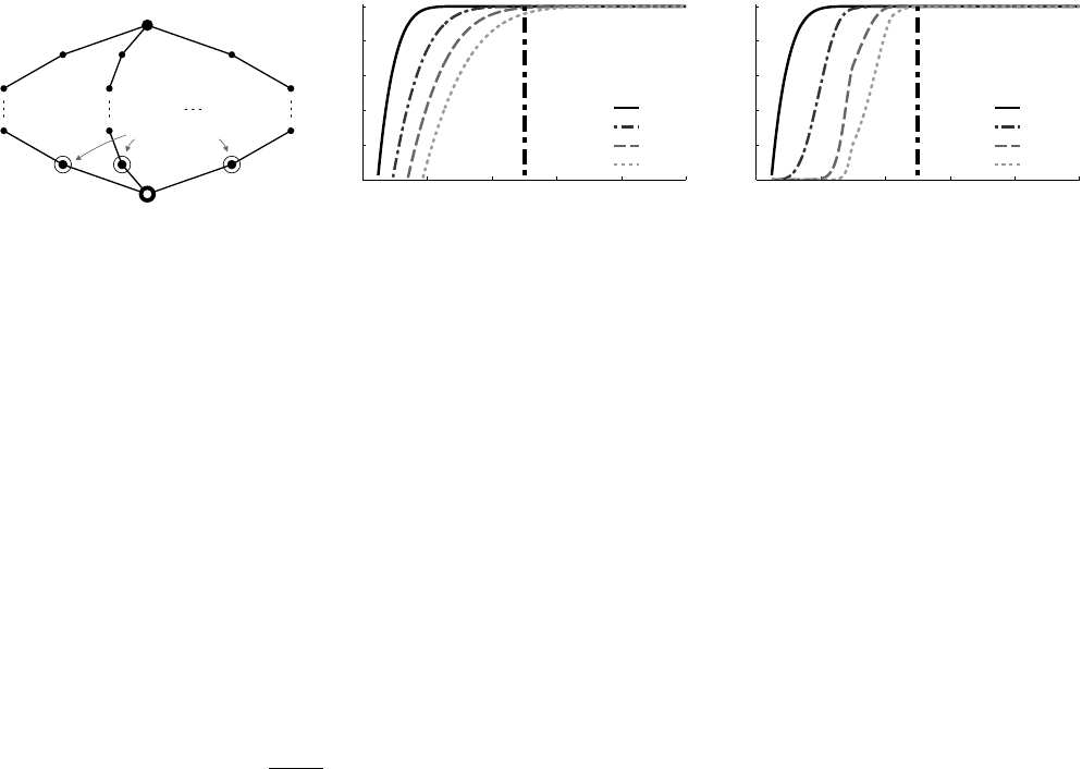
To this end, we consider the network structure in Fig. 10(a).

There are m ≥ 2 independent ﬂooding paths originating at the

initiator. These paths traverse h ≥ 2 hops each, and join again at a

common receiver. In this way, we construct a worst-case scenario in

the sense that the initiator provides the only common synchroniza-

tion point to the paths: nodes on one path relay the ﬂooding packet

independently of nodes on the other paths, which challenges Glossy

in making the ﬁnal m concurrent transmissions interfere construc-

tively at the common receiver.

We ﬁrst present a theoretical model of the temporal displace-

ment ∆ experienced by the common receiver, independent of a spe-

ciﬁc implementation or node platform. Then, we apply this model

to our implementation of Glossy on Tmote Sky devices. The results

show that Glossy generates constructive interference with a proba-

bility above 99.9 % even when 30 nodes transmit concurrently.

6.1 Implementation-independent Analysis

We ﬁrst analyze the sources of temporal uncertainty affecting

the slot length T

slot

given by (1). Our analysis makes use of a mix-

ture of statistical and worst-case assumptions. We consider statisti-

cal distributions for processes that are clearly stochastic in nature,

such as the offset between two unsynchronized clocks. We instead

consider worst-case scenarios for more deterministic variables, in-

cluding clock drift, network topology, and the maximum temporal

displacement among transmitters. Hence, our model provides the

statistical worst-case displacement ∆ experienced by the common

receiver as a function of m and h.

6.1.1 Statistical Uncertainty on Slot Length

We discussed in Sec. 5 that the delay T

introduced by the soft-

ware routine to trigger a transmission is in general not constant,

even if the number of instructions I executed by the MCU is ﬁxed.

The software delay T

is a multiple of the period 1/f

of the crys-

tal sourcing the radio clock. We can thus express the software delay

as T

+ τ

, where

is a constant value corresponding

to the minimum possible delay, and τ

is a discrete random vari-

able with granularity 1/f

representing the additional variation due

to the unsynchronized clocks of the MCU and the radio. We denote

with p

the probability mass function (pmf) of τ

The processing delay of the radio, T

, is also not constant. The

digital circuits of the radio are sourced by a crystal oscillator that

has frequency f

. The radio starts to process an incoming packet

when the digital circuits sampled the beginning of a reception, at

most after 1/f

. We express the processing delay of the radio as

+ τ

. The time needed to process an incoming packet,

is a constant usually in the order of a few microseconds and deter-

mined by the radio. The time required to sample a reception, τ

depends on the offset between the radio clocks of the transmitter

and the receiver. Since these clocks run unsynchronized, τ

is a

random variable with uniform distribution in the interval [0, 1/f

We discretize the set of values of τ

by introducing a time granular-

ity δ such that δ = 1/(k · f

), k  1. Consequently, τ

has uni-

form discrete distribution τ

= {0, δ, 2 · δ, . . . , 1/f

} and pmf p

with constant values 1/(k + 1).

The statistical uncertainty on the length of a slot is the sum of

the uncertainties on the software delay and the radio processing:

slot

= τ

+ τ

(4)

Since δ  1/f

, τ

slot

has granularity δ. The two uncertainties,

and τ

, are independent, because they are due to independent

effects. Recalling that the distribution of the sum of two indepen-

dent random variables can be expressed by their convolution, the

uncertainty on the length of a slot has pmf p

slot

= p

∗ p

6.1.2 Worst-Case Drift of Radio Clock

The time required for a packet transmission, T

, is given by (2)

and depends on the frequency of the radio clock f

. In general,

Common receiver

Initiator

Path 1 Path 2 Path m

m concurrent

transmitters

h − 1

(a) Scenario: a receiver is at the end of

m independent paths of length h.

0 0.2 0.4 0.6 0.8 1

0.0

0.2

0.4

0.6

0.8

1.0

∆

max

= 0.5 µs

Worst−case temporal displacement ∆ [µs]

cdf

h = 2

h = 4

h = 6

h = 8

(b) Distribution of ∆ as a function of network

size h, with m = 2.

0 0.2 0.4 0.6 0.8 1

0.0

0.2

0.4

0.6

0.8

1.0

∆

max

= 0.5 µs

Worst−case temporal displacement ∆ [µs]

cdf

m = 2

m = 5

m = 15

m = 30

sity m, with h = 2.

Figure 10: Scenario and results of the theoretical analysis. In our Glossy implementation, the statistical worst-case temporal displacement

among all transmitters, ∆, is smaller than 0.5 µs with different network settings. Results are provided for N = 3.

this frequency deviates from the nominal value

due to tempera-

ture and aging effects. Crystals used to source the clocks of sensor

network radios have a frequency drift ρ that depends on the tem-

perature t according to a third-order polynomial [26]:

ρ = (f

−

= A(t − t

)

+ B(t − t

) + C (5)

Here, A, B, C, and t

are constants that depend on the speciﬁc

crystal device. Using (5), it is possible to determine bounds on the

frequency drift for a given temperature range.

In the following, we assume −ˆρ ≤ ρ ≤ ˆρ. In the worst case,

among the m independent paths in Fig. 10(a), there is at least one

path where all radio clocks run at the highest frequency

(1 + ˆρ),

and at least one other path where all radio clocks run at the lowest

frequency

(1 − ˆρ). We denote with

the nominal transmission

time in the absence of radio clock drift. With this, we can express

the worst-case variation on the transmission time that accumulates

after h hops at the end of these two independent paths as follows:

= (h − 1) ·

2 · ˆρ

1 − ˆρ

(6)

6.1.3 Statistical Worst-case Temporal Displacement

Each node introduces a statistical uncertainty τ

slot

on the length

of a slot. This uncertainty is independent of other nodes, since

the pair of radio and MCU clocks on one node runs independently

from the pair of clocks on other nodes. Therefore, the temporal

uncertainty τ associated with a path that consists of h hops is the

sum of h−1 independent random variables τ = (h−1)·τ

slot

. The

pmf of τ is given by the convolution of h − 1 instances of p

slot

We now extend the problem to m independent paths, each con-

sisting of h hops and originating at the initiator. We are interested in

the statistical worst-case temporal displacement ∆. This displace-

ment corresponds to the difference between the maximum and the

minimum timing variation associated with each path. We consider

a worst-case scenario where the path with the minimum time varia-

tion has clocks running at the highest frequency, and the path with

the maximum variation has clocks running at the lowest frequency:

∆ = max

[τ] − min

[τ] + τ

(7)

Based on (7), we want to determine the cumulative distribution

function (cdf) of ∆. This corresponds to the problem of ﬁnd-

ing the cdf of the sample range of m independent identically dis-

tributed (i.i.d.) experiments. This is a well-known order statistics

problem, and analytical solutions exist in the literature [2].

6.2 Implementation-dependent Analysis

We now apply the above model to our Glossy implementation on

Tmote Sky devices. We analyze the statistical worst-case temporal

displacement ∆ for different node densities and network sizes. We

use the measurements shown in Fig. 9 to obtain the pmf of the

software delay T

. In addition, we consider ˆρ = 20 ppm as the

maximum drift affecting the radio crystal, which corresponds to a

temperature range between -30°C and 50°C [26].

To analyze the dependency on network size, we ﬁx the number

of paths at m = 2 and vary the path length h between 2 and 8 hops.

Fig. 10(b) plots the cdf of ∆ for four different settings. We see that

∆ is smaller than the requirement of 0.5 µs with very high proba-

bility. This shows that when a ﬂooding packet is relayed along two

independent paths over 8 hops, the two ﬁnal concurrent transmis-

sions generate constructive interference in more than 96 % of the

cases. Recall that this assumes that the time variation due to radio

clock drift is maximum between the two paths. However, in reality,

the drift is usually much smaller than its bounds, which increases

the probability of constructive interference signiﬁcantly.

To analyze the dependency on node density, we set the path

length to h = 2 and vary the number of paths m between 2 and 30.

Fig. 10(c) shows that our Glossy implementation is robust also in

very dense networks. In fact, when 30 nodes transmit concurrently

to a common receiver, ∆ is smaller than 0.5 µs with a probability

above 99.9 %. We show in Sec. 7 that experimental results from

high-density networks conﬁrm these analytical results.

6.3 Theoretical Lower Latency Bound

We provide an expression for the theoretical lower bound on

ﬂooding latency. Intuitively, this bound is given by adding up the

hardware-dependent times for transmitting T

and radio process-

ing T

. Given that nodes transmit concurrently, the theoretical

lower latency bound in a network with size h hops is h· (T

At each hop, Glossy adds a delay T

to the theoretical lower

bound. This delay is introduced by the MCU when issuing a trans-

mission request to the radio. In our implementation, T

is at most

23.5 µs (see Fig. 9). We are not aware of any ﬂooding protocol that

comes so close to the theoretical lower latency bound.

7. EXPERIMENTAL EVALUATION

This section evaluates Glossy on real sensor nodes. We ﬁrst

present results from experiments with a few nodes in several con-

trolled settings. Afterwards, we report on the performance of Glossy

during extensive experiments on three wireless sensor testbeds.

7.1 Glossy in Controlled Experiments

Before evaluating Glossy on several testbeds, we use controlled

experiments to study some of its basic characteristics. We start

by looking at the reliability of concurrent transmissions, deﬁned

as the fraction of packets correctly received by a node. We analyze

how reliability is affected by the temporal displacement ∆ between

0 1 2 3 4 5 6 7 8

100

Reliability [%]

Glossy

∆

max

= 0.5 µs

Temporal displacement ∆ between two concurrent transmitters [µs]

8 bytes

64 bytes

128 bytes

Figure 11: Glossy in a scenario without capture effects, for

N = 1. Reliability is 95 % due to constructive interference when

the temporal displacement ∆ is zero. Reliability drops signiﬁcantly

as ∆ exceeds 0.5 µs, and follows the same pattern as in Fig. 2.

two transmitters and by the total number of concurrent transmitters.

Afterwards, we look at the time synchronization error, which we

deﬁne as the absolute error on the reference time computed by a

receiver with respect to the initiator.

We ﬁnd that (i) Glossy provides a reliability above 95 % in a

scenario where the capture effect does not occur; (ii) while varying

the number of concurrent transmitters between 2 and 10, reliability

stays fairly constant and always above 98 %; (iii) Glossy achieves

an average time synchronization error of less than 0.4 µs even at

receivers that are eight hops away from the initiator.

7.1.1 Impact of Temporal Displacement

The ﬁrst experiment evaluates the reliability of Glossy in a sce-

nario where the capture effect does not occur. In this case, a suc-

cessful reception is only possible if concurrent transmissions inter-

fere constructively. While this is clearly a worst-case scenario that

is difﬁcult to reproduce even under controlled settings, it neverthe-

less gives an indication of Glossy’s robustness.

Setup. We use three nodes, one initiator and two receivers, and

set N = 1. Upon receiving a packet from the initiator, the two

receivers transmit concurrently. The initiator overhears these trans-

missions and records whether it can successfully decode the packet.

Based on sequence numbers embedded in the packets, we measure

the reliability experienced by the initiator. Moreover, we delay the

transmission of one receiver by a variable amount of time in the

interval [0, 8] µs by letting the receiver execute a certain number

of NOPs before issuing a transmission request to the radio. We

set the clock frequency of the MCU to 4 MHz to obtain a temporal

displacement ∆ with 250 ns granularity between the two receivers,

corresponding to half-chip period T

/2 of the modulated signal.

To ensure that the capture effect does not help the initiator in re-

ceiving the packet, we adjust the transmit powers of the receivers.

In particular, we let the non-delayed receiver transmit at -20 dBm,

and the delayed receiver at -13 dBm. In this way, since both sig-

nals are weak and the second one is stronger than the ﬁrst one, we

prevent the initiator from capturing the ﬁrst of the two signals.

Results. Fig. 11 shows reliability for different temporal displace-

ments ∆ and packet lengths, averaged over 2,000 packets for each

setting. We see that the leftmost bar, corresponding to Glossy with-

out artiﬁcial delay, indicates a reliability above 95 % for short pack-

ets. This demonstrates that Glossy makes concurrent transmissions

interfere constructively, allowing a receiver to decode a packet with

very high probability even in the absence of the capture effect. For

increasing ∆ we see a pattern similar to the one in Fig. 2 obtained

through simulation. In particular, reliability starts to drop signif-

icantly at ∆

max

= 0.5 µs, showing local minima when different

chips perfectly overlap. Finally, similar to non-concurrent trans-

missions [25], reliability decreases as packets become longer.

2 3 4 5 6 7 8 9 10

100

Number of concurrent transmitters

Reliability [%]

Figure 12: Reliability depending on number of concurrent

transmitters, including capture effects, for N = 1. Reliability

is fairly constant and always above 98 %, thus showing no signiﬁ-

cant dependency on the number of concurrent transmitters.

1 2 3 4 5 6 7 8

−5

Distance from the initiator [hops]

Time synchroniz. error [µs]

Figure 13: Accuracy of time synchronization in Glossy. The ab-

solute error on the reference time computed by a receiver is below

0.4 µs, even at receivers that are 8 hops apart from the initiator.

7.1.2 Impact of Number of Concurrent Transmitters

In a typical deployment, nodes are not evenly distributed and ex-

perience different channel characteristics. As a result, some nodes

have more neighbors than others. We therefore study in this exper-

iment the impact of the number of transmitters on reliability.

Setup. We use a setup similar to the one above. However, we vary

the number of receivers between 2 and 10, and do not delay their

transmissions artiﬁcially; all packets are 8 bytes long. In this way,

we measure the reliability experienced by the initiator for different

numbers of concurrent transmitters, including capture effects.

Results. Fig. 12 shows reliability, averaged over 10,000 packets for

each setting. We see that reliability stays fairly constant and always

above 98 % as the number of transmitters increases, thus showing

no signiﬁcant dependency between the two. Interestingly, reliabil-

ity is slightly lower when only two or three nodes transmit concur-

rently. In these settings it is more likely that the initiator receives a

weak signal, due to the generation of carriers with slightly different

frequencies or different phases. Our results resemble those in [11],

where nodes transmit ﬁxed-length acknowledgment packets auto-

matically generated by the radio hardware. By contrast, Glossy

transmits variable-length packets generated in software, achieving

even higher reliability in some cases.

7.1.3 Accuracy of Time Synchronization

Glossy provides network-wide time synchronization at no addi-

tional cost. To this end, a receiver computes a reference time when

receiving the ﬁrst ﬂooding packet, as detailed in Sec. 5.4. We as-

sess the accuracy of this computation by looking at the absolute

error with respect to the reference time computed by the initiator.

Setup. We use ﬁve nodes, one initiator and four receivers. At the

beginning of a Glossy phase, the initiator sends a packet, computes

a reference time, and schedules the next phase based on this ref-

erence time. The receivers do exactly the same. After receiving

the packet from the initiator, they compute reference times, and use

these to schedule the beginning of the next phase.

N = 1 N = 2 N = 3 N = 6

Testbed

Tx power Size L R T L R T L R T L R T

[dBm] [hops] [ms] [%] [ms] [ms] [%] [ms] [ms] [%] [ms] [ms] [%] [ms]

MoteLab

(94 nodes)

0 5 1.77 99.37 3.13 1.79 99.88 4.75 1.79 99.96 6.30 1.79 > 99.99 10.87

-7 8 2.28 94.80 4.85 2.35 99.09 5.14 2.37 99.78 6.31 2.39 99.98 10.18

Twist

(92 nodes)

0 3 0.81 99.90 1.99 0.81 > 99.99 3.37 0.81 > 99.99 4.76 0.81 > 99.99 9.07

-15 3 1.18 99.83 2.39 1.18 99.99 3.81 1.18 > 99.99 5.25 1.18 > 99.99 9.60

-25 5 1.74 99.64 3.04 1.75 99.97 4.56 1.75 > 99.99 6.14 1.75 > 99.99 10.84

Local

(39 nodes)

0 3 1.06 99.71 2.31 1.07 99.97 3.76 1.07 > 99.99 5.20 1.07 > 99.99 9.52

-15 7 1.81 98.25 3.45 1.83 99.91 4.75 1.83 99.99 6.26 1.83 > 99.99 10.79

Table 1: Testbed conﬁgurations and results. Tx power is the transmit power of all nodes in a testbed, and size is the corresponding

maximum hop distance between initiator and receivers. We show network-wide averages of ﬂooding latency L, ﬂooding reliability R, and

radio on-time T across four different choices of N, which is the maximum number of transmissions per node during a network ﬂood.

All nodes activate an external pin when a phase starts. We con-

nect the respective pin of the ﬁve nodes to an oscilloscope, moni-

toring the start of a phase at a granularity of 2 ns. Then we measure

the time difference between pin activation at the initiator and pin

activation at the receivers. In this way, we obtain four estimates of

the time synchronization error. To analyze this error for receivers

that are more than one hop away from the initiator, we choose a suf-

ﬁciently large N and let the receivers compute the reference time

based on packets received in later slots.

Results. Fig. 13 shows average and standard deviation of the time

synchronization error depending on hop distance from the initiator,

averaged over 4,000 measurements for each setting. We see that

the average error increases slightly up to hop 3, but then remains as

low as 0.4 µs up to hop 8. The standard deviation increases almost

linearly with hop distance, reaching 4.8 µs at hop 8.

These results show that Glossy achieves accurate time synchro-

nization also at receivers that are several hops away from the initia-

tor. Moreover, they conﬁrm a major result of our theoretical anal-

ysis in Sec. 6, namely that Glossy accumulates only a very small

timing error at each slot. Most of the error is indeed of a stochastic

nature, independent across nodes and different ﬂoods.

7.2 Glossy in Testbed Experiments

Using experiments on three wireless sensor testbeds, we evaluate

Glossy’s performance across several node densities, network sizes,

packet lengths, and transmit powers. The results demonstrate that

Glossy provides robust and efﬁcient network ﬂooding under diverse

conditions. We ﬁrst describe the testbeds and metrics we use. Then

we summarize our key ﬁndings, followed by a detailed discussion

of the experimental results.

7.2.1 Scenario and Metrics

We use three different testbeds to evaluate Glossy: MoteLab [34],

Twist [14], and a local one. These differ along several dimen-

sions, including number of nodes, node density, and network size.

On MoteLab, we collect data from 94 nodes unevenly spread over

three ﬂoors. A node at the corner of the second ﬂoor acts as ini-

tiator. It reaches all other nodes within at most 5 hops when nodes

transmit at the highest power setting of 0 dBm. When transmitting

at -7 dBm, the lowest power that keeps the network fully connected,

the farthest nodes are 8 hops away from the initiator. On Twist, we

use 92 nodes and randomly choose one of them as initiator. Due to

high node density, the network stays connected even at a transmit

power of -25 dBm, yielding a maximum hop distance of 5 from the

initiator. Our local testbed consists of 39 nodes distributed in sev-

eral ofﬁces, passages, and storerooms; two nodes are located out-

side on the rooftop. The initiator reaches all nodes within 7 hops

at the lowest possible transmit power of -15 dBm. On all three

testbeds, we use channel 26 to limit the interference with co-located

WiFi networks. The ﬁrst section in Table 1 lists number of nodes,

transmit powers, and network sizes of each testbed we use.

Our evaluation is based on the following three metrics: (i) ﬂood-

ing latency L of a receiver is the time between the ﬁrst transmission

at the initiator and the ﬁrst successful reception at that receiver;

(ii) ﬂooding reliability R is the fraction of network ﬂoods in which

a receiver successfully receives the packet; (iii) radio on-time T is

the time a receiver has its radio turned on during a network ﬂood.

We compute these metrics for a particular setting based on 50,000

network ﬂoods. We report L, R, and T for each receiver individu-

ally as well as averaged over all receivers in a testbed.

7.2.2 Summary of Testbed Results

Table 1 summarizes the results collected on the three testbeds.

It lists network-wide averages of L, R, and T across four choices

of N. Our experiments reveal the following key ﬁndings:

• The empirical performance of Glossy exhibits no noticeable de-

pendency on node density. Theoretically, performance and node

density are not independent. The analysis in Sec. 6 shows that the

probability of constructive interference is 99.9 % when adding

30 concurrent transmitters. However, we do not discern this

marginal difference in our results from controlled experiments

with up to 10 transmitters (see Sec. 7.1.2) and experiments on

three testbeds, including Twist where nodes are densely deployed.

• The performance of Glossy depends on network size, that is,

on the maximum hop distance between initiator and receivers.

Flooding latency L and radio on-time T increase linearly, and

ﬂooding reliability R decreases logarithmically, as the network

size increases. Nevertheless, for the largest size of 8 hops on

MoteLab with N = 6, L averages around 2.4 ms, R is above

99.9 %, and T is as low as 10.2 ms.

• Increasing the maximum number of transmissions N signiﬁcantly

enhances ﬂooding reliability. For N = 3, we observe that R is at

least 99.9 % across all testbeds and transmit powers except one.

Since R is already very high for N = 1, further increasing N

has no noticeable effect on the average ﬂooding latency. Radio

on-time increases linearly with N, averaging around 16 ms for

the highest value of N = 10 in our experiments.

In the following, we report results from Twist based on network

ﬂoods with an 8-byte packet. This packet length is sufﬁcient to send

short commands to the nodes (e.g., to set system parameters). We

also run experiments with longer packets on MoteLab to see how

the packet length affects the performance of Glossy. We ﬁnd that

ﬂooding reliability decreases logarithmically as the packet length

increases; for example, R is 99.26 % for N = 3 when nodes trans-

mit 128-byte packets at the highest power (see Table 1). This is

expected as current radios make decisions about the correctness of

0 1 2 3 4

0.0

0.2

0.4

0.6

0.8

1.0

Flooding latency [ms]

Fraction of receivers

0 dBm

−15 dBm

−25 dBm

(a) Flooding latency.

99.99 99.992 99.994 99.996 99.998 100

0.0

0.2

0.4

0.6

0.8

1.0

Flooding reliability [%]

Fraction of receivers

0 dBm

−15 dBm

−25 dBm

(b) Flooding reliability.

4 5 6 7 8 9 10

0.0

0.2

0.4

0.6

0.8

1.0

Radio−on time [ms]

Fraction of receivers

0 dBm

−15 dBm

−25 dBm

Figure 14: cdf of Glossy performance on Twist with three different transmit powers, for N = 3.

each individual symbol—a packet is only accepted if all symbols

are correctly received. Flooding latency and radio on-time increase

linearly with packet length since transmissions and receptions take

longer, as described in Sec. 4.2. Overall, the results indicate that

Glossy is suitable for applications that need to ﬂood long packets.

7.2.3 Impact of Network Characteristics

We start by looking at the performance of Glossy under different

network characteristics. To this end, we run experiments with three

different transmit powers on Twist (see Table 1). In doing so, we

effectively control the average node density in the network and the

network size. We keep N = 3 ﬁxed across all runs.

Fig. 14 plots the cdfs of R, L, and T for different transmit pow-

ers. We see from Fig. 14(a) that Glossy needs less than 3 ms to ﬂood

a packet to all 91 receivers, even at the lowest power that merely

keeps the network connected. We are not aware of any current

protocol that provides such fast ﬂooding. We comment on related

ﬂooding and dissemination protocols in Sec. 8.

Looking at Fig. 14(b), we ﬁnd that all receivers have a ﬂood-

ing reliability above 99.99 % at the highest power setting (i.e., at

the highest node density). At the lowest power, still 80 % of the

receivers experience such high reliability. The drop in R is due

to an increased network size. In fact, it takes 5 hops instead of

3 to reach the farthest receivers at the lowest power. This is also

reﬂected in the step-wise shape of the cdf: each step corresponds

to the ﬂooding reliability experienced by receivers at a certain hop

distance from the initiator. This observation conﬁrms also that R

exhibits no noticeable dependency on node density, as hinted by

our controlled experiments in Sec. 7.1.2.

Finally, Fig. 14(c) plots the radio on-time. We see that receivers

listen longer as their hop distance from the initiator increases. Nev-

ertheless, Glossy achieves ultra-low duty cycles also for larger net-

work sizes. For example, consider an application that wants to use

Glossy to (potentially) ﬂood a command every minute. Then, on

Twist, Glossy would utilize not more than 0.01 % of a node’s aver-

age radio duty cycle. We measure comparably low duty cycles on

MoteLab with a maximum distance of 8 hops from the initiator.

7.2.4 Impact of Maximum Number of Transmissions

Next, we analyze how the performance is affected by N, the

maximum number of transmissions per node during a network ﬂood.

We run experiments on Twist and vary N between 1 and 10. To

stress Glossy as much as possible, we use the lowest possible trans-

mit power of -25 dBm, resulting in a network size of 5 hops.

Figs. 15 and 16 plot R, L, and T for different N . Bars show

network-wide averages; error bars indicate the standard deviation.

Flooding reliability, shown in Fig. 15, increases almost logarith-

mically with N . Starting from N = 3, R consistently exceeds

99.99 %. In fact, we performed 50,000 ﬂoods with N = 10, and

only in 3 cases one of the 91 receivers missed the packet.

Flooding latency, shown in Fig. 16, averages around 1.75 ms for

1 2 3 4 5 6 7 8 9 10

99.99999

99.9999

99.999

99.99

99.9

Maximum number of transmissions N

Flooding reliability R [%]

Figure 15: Flooding reliability for various N on Twist. The av-

erage ﬂooding reliability increases almost logarithmically with N.

Within 50,000 network ﬂoods for N = 10, only in 3 cases one of

the 91 receivers missed the packet.

1 2 3 4 5 6 7 8 9 10

Maximum number of transmissions N

Time [ms]

Flooding latency L

Radio−on time T

Figure 16: Flooding latency and radio on-time for various N

on Twist. Radio on-time increases linearly with N , while the aver-

age ﬂooding latency keeps almost constant.

all values of N . It is largely independent of N due to the high

probability of correctly receiving a packet already at the ﬁrst at-

tempt. Given the slot length T

slot

and the relay counter c, we can

compute the ﬂooding latency of a receiver using L = (c+1)·T

slot

assuming perfect reliability.

Finally, by looking at Fig. 16, we see that the radio on-time in-

creases linearly with N. This is also reﬂected in the corresponding

analytical expression T = T

+ 2N · T

slot

, where T

is the time

a receiver listens before the ﬁrst transmission it overhears. The

longest radio on-time averages around 16 ms for N = 10.

8. RELATED WORK

Using Glossy, nodes transmit the same packet concurrently. This

idea stems from work on cooperative communication schemes [28].

However, requirements such as precise time synchronization among

multiple transmitters have long been considered too demanding for

an implementation on real sensor nodes [30].

Flury and Wattenhofer demonstrate the feasibility of signaling

a binary value to all nodes with an unmodulated wave [13]. Con-

structive interference provides the opportunity to extend this to real

data packets. Dutta et al. propose Backcast as an acknowledged

anycast service [11]. Backcast exploits constructive interference of

short acknowledgment packets automatically generated by the ra-

dio hardware. It does not require synchronization among the nodes,

but the application has very limited control over the content of the

interfering packets. In a recent work [10], Backcast serves as the

basis for A-MAC, a receiver-initiated link layer protocol. More-

over, interference has been exploited to increase the throughput of

wireless networks (e.g., through analog network coding [16]).

Flash [21] uses concurrent transmissions for rapid ﬂooding in

sensor networks. Flash relies exclusively on capture effects, which

considerably reduces the chances of correct packet reception when

many nodes transmit concurrently [21]. Glossy also beneﬁts from

capture effects but primarily exploits constructive interference. This

enables Glossy to ﬂood packets with high reliability at any node

density, as demonstrated by our testbed experiments in Sec. 7.2.

Glossy and Flash do not require nodes to maintain information

about the network topology. By contrast, in the Robust Broadcast

Protocol (RBP) [29] and the Collective Flooding (CF) [38] nodes

need to continuously collect information about their local neigh-

borhood to identify links important for the broadcast propagation.

Trickle [19] and its variants provide data dissemination: nodes

continuously send advertisements to detect new data and ensure

complete network coverage. Typically, dissemination protocols are

optimized for reliability and data consistency, not for latency or

energy. Glossy ﬂoods packets fast without additional control trafﬁc,

while sacriﬁcing less than 0.01 % in ﬂooding reliability.

Flooding is a basic communication primitive for time synchro-

nization in sensor networks. For example, the Flooding Time Syn-

chronization Protocol (FTSP) [22] uses periodic ﬂooding of time-

stamped messages and achieves a per-hop synchronization error in

the microsecond range. Lenzen et al. show that optimal synchro-

nization necessitates fast network ﬂooding [18]. Their PulseSync

protocol achieves a higher accuracy than FTSP and a ﬂooding la-

tency below one second. Glossy provides even higher accuracy by

ﬂooding packets within a few milliseconds and employing the Vir-

tual High-resolution Time (VHT) approach by Schmid et al. [27].

The high accuracy and low energy of VHT are also due to the use

of a custom external high-speed crystal [27]. Glossy could enable

further improvements in synchronization accuracy by combining it

with such crystals.

9. CONCLUSIONS

This paper is motivated by real-world sensor network systems

that rely on fast network ﬂooding and accurate time synchroniza-

tion. We observe that such systems would signiﬁcantly beneﬁt from

a service that integrates both functionalities in an efﬁcient man-

ner. This paper thus proposes Glossy, a novel ﬂooding architecture

for wireless sensor networks that uses interference to its advantage.

By making simultaneous transmissions of the same packet interfere

constructively, Glossy enables receivers to decode a packet even in

the absence of capture effects. We have analyzed the robustness

of our techniques in achieving constructive interference based on

a mixture of stochastic and worst-case models. We have evalu-

ated our implementation of Glossy using experiments under con-

trolled settings and on three wireless sensor testbeds. The results

demonstrate that Glossy provides accurate time synchronization

along with fast and highly reliable ﬂooding at ultra-low duty cycles,

showing no noticeable dependency on node density in the scenar-

ios considered. The source code of Glossy is publicly available at

http://www.tik.ee.ethz.ch/~ferrarif/sw/glossy.

Acknowledgments. The authors thank Matthias Keller, Luca Mot-

tola, and Thiemo Voigt for their feedback on early versions of this

paper, and the anonymous reviewers for their helpful comments.

This work was supported by Nano-Tera and the National Compe-

tence Center in Research on Mobile Information and Communi-

cation Systems (NCCR-MICS), a center supported by the Swiss

National Science Foundation under grant number 5005-67322.

10. REFERENCES

[1] The Contiki operating system. http://www.sics.se/contiki/.

[2] B. C. Arnold, N. Balakrishnan, and H. N. Nagaraja. A First Course in Order

Statistics. SIAM, 2008.

[3] Atmel. AT86RF230 datasheet, 2009.

[4] G. Barrenetxea, F. Ingelrest, G. Schaefer, M. Vetterli, O. Couach, and

M. Parlange. SensorScope: Out-of-the-box environmental monitoring. In

ACM/IEEE IPSN, 2008.

[5] J. Choi, M. Kazandjieva, M. Jain, and P. Levis. The case for a network protocol

isolation layer. In ACM SenSys, 2009.

[6] J. Chuang. The effects of time delay spread on portable radio communications

channels with digital modulation. IEEE J. Sel. Areas Commun., 5(5), 1987.

[7] D. Davis and S. Gronemeyer. Performance of slotted ALOHA random access

with delay capture and randomized time of arrival. IEEE Trans. Commun.,

28(5), 1980.

[8] A. Dutta, D. Saha, D. Grunwald, and D. Sicker. SMACK – a SMart

ACKnowledgment scheme for broadcast messages in wireless networks. In

ACM SIGCOMM, 2009.

[9] P. Dutta and D. Culler. Practical asynchronous neighbor discovery and

rendezvous for mobile sensing applications. In ACM SenSys, 2008.

[10] P. Dutta, S. Dawson-Haggerty, Y. Chen, C. M. Liang, and A. Terzis. Design and

evaluation of a versatile and efﬁcient receiver-initiated link layer for low-power

wireless. In ACM SenSys, 2010.

[11] P. Dutta, R. Mus

aloiu-E., I. Stoica, and A. Terzis. Wireless ACK collisions not

considered harmful. In ACM HotNets, 2008.

[12] A. Ephremides and T. Truong. Scheduling broadcasts in multihop radio

networks. IEEE Trans. Commun., 38(4), 1990.

[13] R. Flury and R. Wattenhofer. Slotted programming for sensor networks. In

ACM/IEEE IPSN, 2010.

[14] V. Handziski, A. Köpke, A. Willig, and A. Wolisz. TWIST: A scalable and

reconﬁgurable testbed for wireless indoor experiments with sensor networks. In

ACM REALMAN, 2006.

[15] IEEE. std. 802.15.4-2003, 2003.

[16] S. Katti, S. Gollakota, and D. Katabi. Embracing wireless interference: analog

network coding. In ACM SIGCOMM, 2007.

[17] K. Leentvaar and J. Flint. The capture effect in FM receivers. IEEE Trans.

Commun., 24(5), 1976.

[18] C. Lenzen, P. Sommer, and R. Wattenhofer. Optimal clock synchronization in

networks. In ACM SenSys, 2009.

[19] P. Levis, N. Patel, D. Culler, and S. Shenker. Trickle: A self-regulating

algorithm for code propagation and maintenance in wireless sensor networks. In

USENIX NSDI, 2004.

[20] D. Li, K. Wong, Y. Hu, and A. Sayeed. Detection, classiﬁcation, and tracking of

targets. IEEE Signal Process. Mag., 19(2), 2002.

[21] J. Lu and K. Whitehouse. Flash ﬂooding: Exploiting the capture effect for rapid

ﬂooding in wireless sensor networks. In IEEE INFOCOM, 2009.

[22] M. Maróti, B. Kusy, G. Simon, and A. Lédeczi. The ﬂooding time

synchronization protocol. In ACM SenSys, 2004.

[23] S. Ni, Y. Tseng, Y. Chen, and J. Sheu. The broadcast storm problem in a mobile

ad hoc network. In ACM/IEEE MobiCom, 1999.

[24] M. Rossi et al. SYNAPSE: A network reprogramming protocol for wireless

sensor networks using fountain codes. In IEEE SECON, 2008.

[25] Y. Sankarasubramaniam, I. Akyildiz, and S. McLaughlin. Energy efﬁciency

based packet size optimization in wireless sensor networks. In SNPA, 2003.

[26] T. Schmid. Time in Wireless Embedded Systems. PhD thesis, UCLA, 2009.

[27] T. Schmid, P. Dutta, and M. Srivastava. High-resolution, low-power time

synchronization an oxymoron no more. In ACM/IEEE IPSN, 2010.

[28] B. Sirkeci-Mergen, A. Scaglione, and G. Mergen. Asymptotic analysis of

multistage cooperative broadcast in wireless networks. IEEE Trans. Inf. Theory,

52(6), 2006.

[29] F. Stann, J. Heidemann, R. Shroff, and M. Murtaza. RBP: Robust broadcast

propagation in wireless networks. In ACM SenSys, 2006.

[30] A. Swami, Q. Zhao, and Y. Hong. Wireless Sensor Networks: Signal Processing

and Communications. Wiley, 2007.

[31] Texas Instruments. CC2420 datasheet, 2007.

[32] Texas Instruments. MSP430F1611 datasheet, 2009.

[33] G. Werner-Allen, K. Lorincz, J. Johnson, J. Lees, and M. Welsh. Fidelity and

yield in a volcano monitoring sensor network. In USENIX OSDI, 2006.

[34] G. Werner-Allen, P. Swieskowski, and M. Welsh. MoteLab: A wireless sensor

network testbed. In ACM/IEEE IPSN, 2005.

[35] B. Williams and T. Camp. Comparison of broadcasting techniques for mobile

ad hoc networks. In ACM MobiHoc, 2002.

[36] S. Yoshida and F. Ikegami. A comparison of multipath distortion characteristics

among digital modulation techniques. IEEE Trans. Veh. Technol., 34(3), 1985.

[37] J. Zhao and R. Govindan. Understanding packet delivery performance in dense

wireless sensor networks. In ACM SenSys, 2003.

[38] T. Zhu, Z. Zhong, T. He, and Z.-L. Zhang. Exploring link correlation for

efﬁcient ﬂooding in wireless sensor networks. In USENIX NSDI, 2010.