
A Survey of Generalized Gauss-Newton and
Sequential Convex Programming Methods
Moritz Diehl
Systems Control and Optimization Laboratory
Department of Microsystems Engineering and Department of Mathematics
University of Freiburg, Germany
based on joint work with
Florian Messerer (Freiburg)
and Joris Gillis (Leuven)
19th French-German-Swiss Conference on Optimization, Nice,
September 18, 2019
1 / 42

A Tutorial of Generalized Gauss-Newton and
Sequential Convex Programming Methods
Moritz Diehl
Systems Control and Optimization Laboratory
Department of Microsystems Engineering and Department of Mathematics
University of Freiburg, Germany
based on joint work with
Florian Messerer (Freiburg)
and Joris Gillis (Leuven)
19th French-German-Swiss Conference on Optimization, Nice,
September 18, 2019
2 / 42

Nonlinear optimization with convex substructure
minimize
w ∈ R
n
w
φ
0
(F
0
(w))
subject to F
i
(w) ∈ Ω
i
i = 1, . . . , m,
G(w) = 0
Assumptions:
twice continuously differentiable functions G : R
n
w
→ R
n
g
and
F
i
: R
n
w
→ R
n
F
i
for i = 0, 1, . . . , m.
outer function φ
0
: R
n
F
0
→ R convex.
sets Ω
i
⊂ R
n
F
i
convex for i = 1, . . . , m,
(possibly z ∈ Ω
i
⇔ φ
i
(z) ≤ 0 with smooth convex φ
i
)
Idea:
exploit convex substructure via iterative convex approximations.
3 / 42

Why is this class of problems and algorithms interesting?
some nonlinear programming (NLP) problems have nonsmooth
convex constraints which cannot be treated by standard NLP solvers
there exist many reliable and efficient convex optimization solvers
Some application areas:
nonlinear matrix inequalities for reduced order controller design
[Fares, Noll, Apkarian 2002; Tran-Dinh et al. 2012]
ellipsoidal terminal regions in nonlinear model predictive control
[Chen and Allg¨ower 1998; Verschueren 2016]
robustified inequalities in nonlinear optimization [Nagy and Braatz
2003; D., Bock, Kostina 2006]
tube-following optimal control problems [Van Duijkeren, 2019]
non-smooth composite minimization [Lewis and Wright 2016]
deep neural network training with convex loss functions
[Schraudolph 2002; Martens 2016]
4 / 42

First the bad news
Iterative convex approximation methods such as sequential convex
programming (SCP) have only linear convergence in general.
The rate of convergence cannot be improved to superlinear by any
bounded semi-definite Hessian approximation [D., Jarre, Vogelbusch
2006]
Simple TR example problem with dominant nonconvexities in objective:
minimize
w ∈ R
2
− w
2
1
− (1 − w
2
)
2
subject to kwk
2
≤ 1
But: many real-world problems have dominant convexities and SCP often
shows fast linear convergence in practice. How fast?
5 / 42

First the bad news
Iterative convex approximation methods such as sequential convex
programming (SCP) have only linear convergence in general.
The rate of convergence cannot be improved to superlinear by any
bounded semi-definite Hessian approximation [D., Jarre, Vogelbusch
2006]
Simple TR example problem with dominant nonconvexities in objective:
minimize
w ∈ R
2
− w
2
1
− (1 − w
2
)
2
subject to kwk
2
≤ 1
But: many real-world problems have dominant convexities and SCP often
shows fast linear convergence in practice.
How fast?
5 / 42

First the bad news
Iterative convex approximation methods such as sequential convex
programming (SCP) have only linear convergence in general.
The rate of convergence cannot be improved to superlinear by any
bounded semi-definite Hessian approximation [D., Jarre, Vogelbusch
2006]
Simple TR example problem with dominant nonconvexities in objective:
minimize
w ∈ R
2
− w
2
1
− (1 − w
2
)
2
subject to kwk
2
≤ 1
But: many real-world problems have dominant convexities and SCP often
shows fast linear convergence in practice. How fast?
5 / 42

Overview
Smooth unconstrained problems
Sequential Convex Programming (SCP)
Generalized Gauss-Newton (GGN)
Local convergence analysis
Desirable divergence
Illustrative example in CasADi
Constrained problems
Sequential Convex Programming (SCP)
Sequential Linear Programming (SLP)
Constrained Generalized Gauss-Newton (CGGN)
Sequential Convex Quadratic Programming (SCQP)
Recent Progress in Dynamic Optimization and Applications
6 / 42

Simplest case: smooth unconstrained problems
Unconstrained minimization of ”convex over nonlinear” function:
minimize
w ∈ R
n
φ(F (w))
| {z }
=:f(w)
Assumptions:
- Inner function F : R
n
→ R
N
of class C
3
- Outer function φ : R
N
→ R of class C
3
and convex
Remark:
F, φ, f ∈ C
3
avoids technical details that would obfuscate main results.
7 / 42

Notation and Preliminaries
Matrix inequality A B for A, B ∈ S
n
(symmetric matrices)
Gradient ∇f(w) ∈ R
n
and Hessian ∇
2
f(w) ∈ S
n
for f : R
n
→ R
Jacobian J(w) :=
∂F
∂w
(w) ∈ R
N×n
for F : R
n
→ R
N
Linearization (first order Taylor series) at ¯w ∈ R
n
:
F
lin
(w; ¯w) := F ( ¯w) + J( ¯w) (w − ¯w)
Big O(·) notation: e.g. F
lin
(w; ¯w) = F (w) + O(kw − ¯wk
2
)
Note: gradient of f(w) = φ(F (w)) is ∇f (w) = J(w)
>
∇φ(F (w))
8 / 42

Method 1: Sequential Convex Programming (SCP)
Starting at w
0
∈ R
n
we generate sequence . . . , w
k
, w
k+1
, . . .
by obtaining w
k+1
as solution of convex subproblem at ¯w = w
k
:
minimize
w ∈ R
n
φ (F
lin
(w; ¯w))
| {z }
=:f
SCP
(w; ¯w)
(1)
(requires possibly expensive calls of a convex optimization solver)
Observation: f
SCP
(w; ¯w) = f (w) + O(kw − ¯wk
2
)
Corollary: ∇f( ¯w) = 0 ⇔ ¯w fixed point of SCP
(if subproblems (1) have unique solutions)
9 / 42

Tutorial Example
Regard F (w) =
sin(w)
exp(w) − 2
and φ(z) = z
4
1
+ z
2
2
Linearization: F
lin
(w; ¯w) =
sin( ¯w) + cos( ¯w)(w − ¯w)
exp( ¯w) − 2 + exp( ¯w)(w − ¯w)
SCP objective:
f
SCP
(w; ¯w) = (sin( ¯w)+cos( ¯w)(w− ¯w))
4
+
(exp( ¯w)−2+exp( ¯w)(w− ¯w))
2
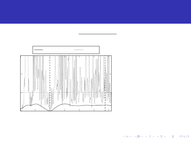
Fig.: f(w) = φ(F (w)) (solid) and f
SCP
(w; ¯w) (dashed) for ¯w = 0
10 / 42

SCP for Least Squares Problems = Gauss-Newton
With quadratic φ(z) =
1
2
kzk
2
2
=
1
2
z
>
z, SCP subproblems become
minimize
w ∈ R
n
1
2
kF (w
k
) + J(w
k
)(w − w
k
)k
2
2
(2)
If rank(J) = n this is uniquely solvable, giving
w
k+1
= w
k
−
J(w
k
)
>
J(w
k
)
| {z }
=:B
GN
(w
k
)
−1
J(w
k
)
>
F (w
k
)
| {z }
=∇f(w
k
)
SCP applied to LS = Newton method with ”Gauss-Newton Hessian”
B
GN
(w) ≈ ∇
2
f(w)
11 / 42

Method 2: Generalized Gauss-Newton cf. [Schraudolph 2002]
For general convex φ(·) we have for f(w) = φ(F (w))
∇
2
f(w) = J(w)
>
∇
2
φ(F (w)) J(w)
| {z }
=:B
GGN
(w)
”GGN Hessian”
+
P
N
j=1
∇
2
F
j
(w) ∇
z
j
φ(F (w))
| {z }
=:E
GGN
(w)
”Error matrix”
Generalized Gauss-Newton (GGN) method iterates according to
w
k+1
= w
k
− B
GGN
(w)
−1
∇f(w
k
)
Note: GGN solves convex quadratic subproblems
min
w ∈R
n
f(w
k
)+∇f(w
k
)
>
(w−w
k
)+
1
2
(w−w
k
)
>
B
GGN
(w
k
)(w−w
k
)
| {z }
=:f
GGN
(w;w
k
)
12 / 42


Differences and Similarities of SCP and GGN
both SCP and GGN generalize the Gauss-Newton method
(and become equal to it when applied to nonlinear least squares)
both iteratively solve convex optimization problems
GGN only solves a positive definite linear system per iteration
SCP solves a full convex problem per iteration (5-30x slower)
SCP often less sensitive to initialization
both are NOT second order methods
both converge linearly with the same rate (details follow)
14 / 42

Local Convergence Analysis for SCP and GGN
Recall:
f
SCP
(w; ¯w) = φ (F
lin
(w; ¯w))
f
GGN
(w; ¯w) = f ( ¯w)+∇f( ¯w)
>
(w− ¯w)+
1
2
(w− ¯w)
>
B
GGN
( ¯w)(w− ¯w)
∇
w
f
SCP
( ¯w; ¯w) = ∇
w
f
GGN
( ¯w; ¯w) = ∇f( ¯w)
Lemma 1 (Equality of SCP and GGN up to Second Order)
f
SCP
(w; ¯w) = f
GGN
(w; ¯w) + O(kw − ¯wk
3
)
Proof: ∇
2
w
f
SCP
( ¯w; ¯w) = B
GGN
( ¯w) = ∇
2
w
f
GGN
( ¯w; ¯w)
Note: in general B
GGN
( ¯w) 6= ∇
2
f( ¯w)
15 / 42

Local Convergence of SCP and GGN
Main Theorem 1 [Diehl and Messerer, CDC 2019]
Regard w
∗
with ∇f(w
∗
) = 0 and B
GGN
(w
∗
) 0. Then
w
∗
is a fixed point for both the SCP and GGN iterations
both methods are well-defined in a neighborhood of w
∗
their linear contraction rates are equal and given by the LMI
min{α ∈ R | − αB
GGN
(w
∗
) E
GGN
(w
∗
) αB
GGN
(w
∗
)}
Corollary: Necessary condition for local convergence of both methods is
B
GGN
(w
∗
)
1
2
∇
2
f(w
∗
) 0
*Proof of corollary: Set α =1 and use E
GGN
(w
∗
)= ∇
2
w
f(w
∗
)−B
GGN
(w
∗
)
16 / 42

*Proof of Main Theorem
Define solution operators w
sol
SCP
( ¯w) and w
sol
GGN
( ¯w) at linearization point
¯w and apply the implicit function theorem to
∇
w
f
i
(w
sol
i
( ¯w); ¯w) = 0 for i = SCP, GGN
Well-defined for ¯w in neighborhood of w
∗
because
∇
2
w
f
SCP
(w
∗
; w
∗
) = ∇
2
w
f
GGN
(w
∗
; w
∗
) = B
GGN
(w
∗
) 0, and derivatives
are given by
dw
sol
i
d ¯w
(w
∗
) = −(∇
w
∇
w
f
i
(w
∗
; w
∗
)
| {z }
=B
GGN
(w
∗
)=:B
∗
)
−1
∇
¯w
∇
w
f
i
(w
∗
; w
∗
)
| {z }
=E
GGN
(w
∗
)=:E
∗
We used that all second derivatives are equal due to Lemma 3 and that
∇
¯w
∇
w
f
GGN
(w
∗
; w
∗
) = ∇
¯w
(∇f( ¯w) + B
GGN
( ¯w)(w − ¯w))|
w= ¯w=w
∗
= ∇
2
f(w
∗
) − B
GGN
(w
∗
) = E
GGN
(w
∗
)
17 / 42

*Proof of Main Theorem (continued)
Spectral radius ρ(−B
−1
∗
E
∗
) = ρ(B
−1
∗
E
∗
) equals linear contraction rate
of SCP and GGN algorithms. Matrix can be transformed to similar, but
symmetric matrix: B
−1
∗
E
∗
∼ B
−
1
2
∗
E
∗
B
−
1
2
∗
with same spectral radius.
Now, ρ(B
−
1
2
∗
E
∗
B
−
1
2
∗
) ≤ α ⇔ −αI B
−
1
2
∗
E
∗
B
−
1
2
∗
αI
⇔ −αB
∗
E
∗
αB
∗
18 / 42

Desirable divergence and mirror problem, cf. [Bock 1987]
SCP and GGN do not converge to every local minimum. This can help to
avoid ”bad” local minima, as discussed next.
Regard maximum likelihood estimation problem min
w
φ(M(w) − y)
with nonlinear model M : R
n
→ R
N
and measurements y ∈ R
N
.
Assume penalty φ is symmetric with φ(−z) = φ(z) as is the case for
symmetric error distributions. At a solution w
∗
, we can generate ”mirror
measurements” y
mr
:= 2M(w
∗
) − y obtained by reflecting the residuals.
From a statistical point of view, y
mr
should be as likely as y.
19 / 42

SCP Divergence ⇔ Minimum unstable under mirroring
Theorem 2 [Diehl and Messerer 2019] generalizing [Bock 1987]
Regard a local minimizer w
∗
of f(w) = φ(M(w) − y) with
∇
2
f(w
∗
) 0. If the necessary SCP-GGN-convergence condition
B
GGN
(w
∗
)
1
2
∇
2
f(w
∗
) does not hold, then w
∗
is a stationary point of
the mirror problem but not a local minimizer.
*Sketch of proof: use M (w
∗
) − y
mr
= y − M (w
∗
) to show that
∇f
mr
(w
∗
) = J(w
∗
)
>
(y − M (w
∗
)) = 0 and
∇
2
f
mr
(w
∗
) = B
GGN
(w
∗
) − E
GGN
(w
∗
) = 2B
GGN
(w
∗
) − ∇
2
f(w
∗
) 6 0
20 / 42

Illustrative example (experiments conducted by Florian Messerer)
0 2 4 6 8
−1
0
1
input x
output
y
m(x, w
true
)
Regard scalar model with unknown parameter w
m(x, w) := sin(wx)
with input output measurements (x
i
, y
i
) for i = 1, . . . , N (left plot).
Define M
i
(w) := m(x
i
, w) and F (w) := M(w) − y
As outer convexity we use a Huber-like penalty (right plot)
φ(z) :=
1
N
N
X
i=1
q
δ
2
+ z
2
i
, (3)
21 / 42

Implementation of SCP and GGN
obtain all needed derivatives from CasADi via MATLAB interface
use linear solve (”backslash”) for GGN
formulate SCP subproblem as second order cone program (SOCP):
min
w ∈ R,
s ∈ R
N
N
X
i=1
s
i
s.t.
q
δ
2
+ F
lin,i
(w; w
k
)
2
≤ s
i
for i = 1, . . . , N
use Gurobi via CasADi as SOCP solver
22 / 42

CasADi for Optimization Modelling
●
A software framework for nonlinear optimization and optimal control
●
“Write an efficient optimal control solver in a few lines”
●
Implements automatic differentiation (AD) on sparse matrix-valued
computational graphs in C++11
●
Front-ends to Python, Matlab and Octave
●
Supports C code generation
●
Back-ends to SUNDIALS, CPLEX, Gurobi, qpOASES, IPOPT, KNITRO,
SNOPT, SuperSCS, OSQP, …
●
Developed by Joel Andersson and Joris Gillis
http://casadi.org
Nov 18-20: Hands-on CasADi course on optimal control: http://hasselt2019.casadi.org
Jupyter CasADi demo for this talk: http://fgs.casadi.org
23 / 42


Overview
Smooth unconstrained problems
Sequential Convex Programming (SCP)
Generalized Gauss-Newton (GGN)
Local convergence analysis
Desirable divergence
Illustrative example in CasADi
Constrained problems
Sequential Convex Programming (SCP)
Sequential Linear Programming (SLP)
Constrained Generalized Gauss-Newton (CGGN)
Sequential Convex Quadratic Programming (SCQP)
Recent Progress in Dynamic Optimization and Applications
28 / 42


Sequential Linear Programming (SLP)
If functions φ
0
, . . . , φ
m
are linear, SCP just solves linear programs (LP):
minimize
w ∈ R
n
w
f
lin
0
(w; ¯w)
subject to f
lin
i
(w; ¯w) ≤ 0, i = 1, . . . , m,
G
lin
(w; ¯w) = 0
might be called Sequential Linear Programming (SLP)
(”Method of Approximation Programming” by Griffith & Stewart, 1961)
equivalent to standard SQP with zero Hessian
SLP only attracted to NLP solutions in vertices of feasible set
works very well for L1-estimation [Bock, Kostina, Schl¨oder 2007]
converges quadratically once correct active set is discovered
31 / 42

Picture from Griffith and Stewart’s original 1961 paper
386 R. E. GRIFFITH AND R. A. STEWART
y
5-
4-
>i.P SOLUTION
STARTING
31 | ~~~~~P O I N T TR UE d
o'I 3
FIG. 4. Third LP problem
For the purpose of illustration we will consider the problem of balancing cata-
lytic reformer severity (S) with tetraethyl lead (TEL) level in gasoline blending.
We will simplify the problem to the following.
A catalytic reformer is a plant which can increase the octane number (ON)
of a gasoline stream but only with an associated loss in volume of the gasoline
stream. The only operating variable considered here is a severity parameter (S).
The by-products from this reformer operation are not gasoline components but
may be sold at a fixed unit price. The total value of the by-products will be
(VBP). The operating cost (OC) of running the reformer is a function of S. The
main product of the reformer is called reformate (R). The reformer has a fixed
amount of feed which must be processed and all the reformate must be blended.
TEL is a material which may be added to gasoline to increase the ON. TEL
does not change the volume of the gasoline.
Two blends of gasoline are required in this problem, premium (A) and regular
(B). There is a maximum amount of premium which may be blended but no
quantity restriction is placed on the regular.
The only quality specification considered here is ON. Both blends A and B
must meet a minimum ON.
This content downloaded from 46.183.103.17 on Thu, 21 Mar 2019 20:34:26 UTC
All use subject to https://about.jstor.org/terms
32 / 42

Constrained Generalized Gauss-Newton [Bock 1987]
Use B
GGN
(w) := J
0
(w)
>
∇
2
φ
0
(F
0
(w))J
0
(w) and solve convex quadratic
program (QP)
minimize
w ∈ R
n
w
f
lin
0
(w; ¯w) +
1
2
(w − ¯w)
>
B
GGN
( ¯w)(w − ¯w)
subject to f
lin
i
(w; ¯w) ≤ 0, i = 1, . . . , m,
G
lin
(w; ¯w) = 0
like SCP, the method is multiplier free
also affine invariant
Remark: for least-squares objectives, this method is due to [Bock 1987]. In
mathematical optimization papers, Bock’s method is called ”the Generalized
Gauss-Newton (GGN) method” because it generalizes the GN method to
constrained problems. To avoid a notation clash with computer science we
prefer to call Bock’s method ”the Constrained Gauss-Newton (CGN) method”.
33 / 42

Sequential Convex Quadratic Programming (SCQP) [Verschueren et al. 2016]
B
SCQP
(w, µ) := J
0
(w)
>
∇
2
φ
0
(F
0
(w))J
0
(w) +
m
X
i=1
µ
i
J
i
(w)
>
∇
2
φ
i
(F
i
(w))J
i
(w)
minimize
w ∈ R
n
w
f
lin
0
(w; ¯w) +
1
2
(w − ¯w)
>
B
SCQP
( ¯w, ¯µ)(w − ¯w)
subject to f
lin
i
(w; ¯w) ≤ 0, i = 1, . . . , m, | µ
+
,
G
lin
(w; ¯w) = 0
again, only a QP needs to be solved in each iteration
again, affine invariant
”optimizer state” contains both, ¯w and inequality multipliers ¯µ
B
SCQP
(w, µ) B
GGN
(w) i.e. more likely to converge than GGN
SCQP has same contraction rate as SCP, characterized by two LMI on the
reduced Hessian approximation [Messerer &D., 2019]
34 / 42

Overview
Smooth unconstrained problems
Sequential Convex Programming (SCP)
Generalized Gauss-Newton (GGN)
Local convergence analysis
Desirable divergence
Illustrative example in CasADi
Constrained problems
Sequential Convex Programming (SCP)
Sequential Linear Programming (SLP)
Constrained Generalized Gauss-Newton (CGGN)
Sequential Convex Quadratic Programming (SCQP)
Recent Progress in Dynamic Optimization and Applications
35 / 42

Dynamic Optimization in a Nutshell
minimize
x, u
N
X
i=0
ϕ
i
(F
i
(x
i
, u
i
)) + ϕ
N
(F
N
(x
N
))
subject to x
i+1
= S
i
(x
i
, u
i
), i = 0, . . . , N − 1,
H
i
(x
i
, u
i
) ∈ Ω
i
, i = 0, . . . , N − 1,
H
N
(x
N
) ∈ Ω
N
variables w = (x, u) with x = (x
0
, . . . , x
N
) and u = (u
0
, . . . , u
N −1
)
convexities in ϕ
i
(e.g. quadratic) and Ω
i
(e.g. polyhedral)
nonlinearities in dynamic system S
i
and constraint functions F
i
, H
i
often: S
i
result of time integration (direct multiple shooting)
36 / 42

Recent Algorithmic Progress
Inexact Newton with Iterated Sensitivities (INIS) - Rien Quirynen
Generalized Nonlinear Static Feedback Integration - Jonathan Frey
Zero Order Moving Horizon Estimation - Katrin Baumg¨artner
Advanced Step Real-Time Iteration - Armin Nurkanovic
Convex Inner Approximation (CIAO) for mobile robots - Tobias Sch¨ols
37 / 42

Recent Progress on Software and Applications
BLASFEO: BLAS for Embedded Optimization - Gianluca Frison
acados: real-time SCQP type algorithms for nonlinear model predictive
control (NMPC) - Robin Verschueren, Dimitris Kouzoupis, Gianluca
Frison, et al.
(both under permissive open-source BSD license)
Recent real-world NMPC applications:
NMPC of small quadcopters in Freiburg - Barbara Barrros
NMPC of human sized quadcopters in California - Andrea Zanelli
4 kHz NMPC of reluctance synchronous motor in Munich - Andrea Zanelli
100 Hz NMPC of Freiburg race cars - Daniel Kloeser
10 Hz CIAO-NMPC of mobile robots at Bosch - Tobias Sch¨ols
38 / 42


Conclusions
Discussed a family of Iterative Convex Approximation Methods
Sequential Convex Programming (SCP) conceptually simplest
(”linearize nonlinearities, keep all convex structures”) and most
widely applicable e.g. to nonlinear cone programming.
Generalized Gauss-Newton (GGN) cheaper iterations as only QPs
are solved. Unconstrained GGN and constrained SCQP show
identical local convergence rates as SCP for smooth problems.
Local contraction rate for both SCP and GGN equals smallest α
satisfying −αB
GGN
(w
∗
) ∇
2
f(w
∗
) − B
GGN
(w
∗
) αB
GGN
(w
∗
)
Divergence might in fact be a desirable property in estimation as it
avoids being attracted by statistically unstable local minima
40 / 42

Some References 1
J. Andersson, J. Gillis, G. Horn, J. B. Rawlings, and M. Diehl. CasADi: a
software framework for nonlinear optimization and optimal control.
Mathematical Programming Computation, 2018.
H.G. Bock, E. Kostina, and J.P. Schl¨oder. Numerical methods for
parameter estimation in nonlinear differential algebraic equations. GAMM
Mitteilungen, 30/2:376-408, 2007.
J. Martens. Second-Order Optimization for Neural Networks. PhD thesis,
University of Toronto, 2016.
N. Schraudolph. Fast curvature matrix-vector products for second-order
gradient descent. Neural Computation, 14(7):1723–1738, 2002.
Q. Tran-Dinh. Sequential Convex Programming and Decomposition
Approaches for Nonlinear Optimization. PhD thesis, KU Leuven, 2012.
R. Verschueren, N. van Duijkeren, R. Quirynen, and M. Diehl. Exploiting
convexity in direct optimal control: a sequential convex quadratic
programming method. In Proceedings of the IEEE Conference on Decision
and Control (CDC), 2016.
41 / 42

Some References 2
M. Diehl and F. Messerer. Local Convergence of Generalized
Gauss-Newton and Sequential Convex Programming, CDC, 2019
(accepted)
N. Van Duijkeren. Online Motion Control in Virtual Corridors for Fast
Robotic Systems, PhD thesis, KU Leuven, 2019.
M. Diehl, F. Jarre, C. Vogelbusch. Loss of superlinear convergence for an
SQP-type method with conic constraints, SIAM Journal on Optimization,
2006.
Q. Tran-Dinh, S. Gumussoy, W. Michiels, M. Diehl. Combining
convex-concave decompositions and linearization approaches for solving
BMIs, with application to static output feedback, IEEE Transactions on
Automatic Control, 2012.
R.E. Griffith and R.A. Stewart. A Nonlinear Programming Technique for
the Optimization of Continuous Processing Systems, Management Sci., 7:
379-392, 1961.
42 / 42
